Multiplexing and Traffic Engineering

Multiplexing

Multiplexing combines several low-capacity signals onto one high-capacity transmission medium; demultiplexing separates the composite back into individual channels at the far end.

Sharing a transmission system avoids a separate cable, radio link, or repeater chain for every channel. The aggregate link must still provide enough usable capacity for the tributaries and multiplexing overhead.

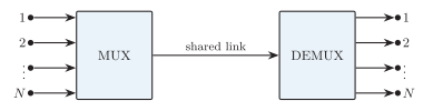
Multiplexing and demultiplexing system.

Space Division Multiplexing

Note

Note

Space-Division Multiplexing (SDM) is a telecommunication technique that increases the data-carrying capacity of a communication channel by transmitting multiple independent data streams simultaneously across physically or spatially separated paths. Unlike techniques that divide time or frequency, SDM utilizes the physical dimension of space to create parallel transmission lanes.

Working Principle

SDM operates on the concept of spatial isolation. Instead of forcing multiple signals to share the exact same physical path, the medium is structurally configured to provide distinct, independent routes. Because the signals travel along separate spatial paths, they do not inherently overlap or interfere with one another, allowing the entire system bandwidth to be multiplied by the number of spatial paths available.

Implementation Methods

In modern networks, SDM is deployed using different physical architectures:

• Multi-Core Fibers (MCF): Packing multiple glass cores into a single optical fiber cable, where each core acts as a distinct data highway.

• Mode-Division Multiplexing (MDM): Sending multiple signals down a single fiber core by shaping the light into different spatial modes or geometrical paths that do not mix.

• Multi-Antenna Arrays (MIMO): In wireless systems (like 4G/5G), using Multiple-Input Multiple-Output spatial antennas to send different data streams through the air using the exact same frequency block.

Technical Comparison

While Frequency-Division Multiplexing (FDM) splits a channel by broadcasting on different frequencies, and Time-Division Multiplexing (TDM) splits a channel by assigning specific time slots, SDM splits the physical infrastructure itself to handle separate signals.

Importance & Core Challenge

• Importance: SDM is crucial for overcoming the “capacity crunch” in fiber optics. Traditional fibers are reaching their absolute physical data limits; SDM allows exponential bandwidth growth without laying down entirely new cables.

• Challenge: The main drawback is crosstalk (signal leakage between tightly packed spatial paths), which requires advanced Digital Signal Processing (DSP) techniques at the receiving end to untangle and clean the data.

Frequency Division Multiplexing (FDM)

Definition and Operating Principle

Frequency-Division Multiplexing (FDM) divides the total bandwidth of a shared transmission medium into separate, non-overlapping frequency channels. Each input signal is assigned a different carrier frequency, so all channels are transmitted continuously and simultaneously.

At the transmitter, each message signal $m_i(t)$ modulates its assigned carrier $f_i$ to form a channel signal $s_i(t)$. The multiplexer adds the $N$ channel signals to produce the composite FDM signal

$$x(t)=\sum_{i=1}^{N}s_i(t),$$

where $x(t)$ is transmitted over the common medium. The carrier frequencies are spaced so that the channel spectra do not overlap.

Transmitter and Receiver Operation

1. Modulation: Each input signal modulates a carrier at a different frequency, placing it in an allocated frequency channel.

2. Combining: The modulated channel signals are added to form one composite signal and transmitted over the shared medium.

3. Separation: At the receiver, a bank of bandpass filters (BPFs) selects the required frequency channel.

4. Recovery: A demodulator converts the selected channel back to its original message signal.

Unlike TDM, FDM does not require time-slot or frame synchronisation; correct separation depends mainly on frequency allocation and filtering.

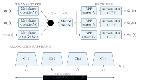
FDM modulation, channel allocation, and receiver filter-bank recovery.

Guard Bands and Spectral Efficiency

Guard bands are small unused frequency gaps placed between adjacent channels. They are required because practical filters do not have perfectly sharp cut-offs and carrier frequencies may vary slightly. Wider guard bands reduce adjacent-channel interference but waste more bandwidth; narrower guard bands improve spectral efficiency but require better filtering and frequency stability.

Core Advantages and Limitations

Advantages

• Continuous, real-time transmission by every channel.

• No time-slot or frame synchronisation is required.

• Well suited to analog and broadcast services.

• All channels can carry signals simultaneously.

Disadvantages

• Guard bands consume usable spectrum.

• Requires modulators and selective bandpass filters.

• Fixed channel allocation wastes capacity when a channel is idle.

• Poor filtering may cause adjacent-channel interference.

Practical Applications

• Radio and television broadcasting: Stations occupy separate assigned carrier-frequency channels in the shared radio spectrum.

• Cable television (CATV): Many television and data channels travel concurrently over one coaxial cable.

• Carrier telephony and satellite/microwave links: Voice or data tributaries are translated into separate channels within a wideband trunk or transponder.

• First-generation cellular systems: The same frequency-partitioning principle was used as FDMA, assigning one radio channel to each active call.

Time Division Multiplexing (TDM)

TDM lets several signals share one channel by assigning each a separate time slot. Only one user transmits per slot, but slots repeat rapidly so communication appears continuous apparently.

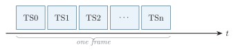
TDM frame structure.

Types of TDM

Type	Description	Example
Synchronous	Fixed slot per channel, even if idle	PCM, E1/T1
Statistical (also called asynchronous TDM)	Capacity assigned to active sources; labels identify destinations and buffering absorbs bursts	Data multiplexers, packet links

PCM-TDM Rate

Conventional telephony limits speech to about $3.4\,\mathrm{kHz}$ and samples at $8\,\mathrm{kHz}$. G.711 PCM represents each sample with 8 bits, producing a $64\,\mathrm{kbit/s}$ channel.

Note

PCM voice channel rate

$$R_{\text{voice}}=8000\times8=64\,kbit/s.$$

An E1 system multiplexes $32$ such slots:

$$32\times64\,kbit/s=2.048\,Mbit/s.$$

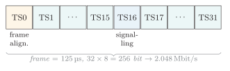
E1/PCM-30 frame structure.

An E1 frame contains 32 eight-bit time slots every $125\,\mu\mathrm{s}$. In PCM-30, TS0 carries frame alignment and related overhead, TS16 carries signalling, and the other 30 slots carry bearer channels. Channel-associated signalling uses TS16 over a 16-frame multiframe; E1 configurations without this signalling reservation can allocate slots differently.

Advantages and Disadvantages

Advantages

• Efficient for digital signals.

• No guard bands are needed.

• Easy integration with digital switching.

Disadvantages

• Requires synchronisation.

• Idle slots waste capacity in synchronous TDM.

• Timing jitter degrades quality.

Wavelength Division Multiplexing (WDM)

Note

Wavelength-Division Multiplexing (WDM)

is an optical multiplexing technology that transmits multiple independent data streams simultaneously over one optical fibre by assigning each stream a different wavelength (colour) of laser light.

• WDM is the optical counterpart of FDM. It increases the capacity of existing fibre infrastructure without installing additional fibres, provided that the optical spectrum, equipment, and link budget support the extra wavelength channels.

Core Principles and Architecture

1. Multiplexing (MUX): Optical transmitters or transponders carry separate data streams on distinct wavelengths $\lambda_1,\ldots,\lambda_n$. An optical multiplexer combines them into one composite light signal.

2. Transmission: The combined wavelengths propagate through the same fibre core. Channel spacing and optical filtering keep the streams distinguishable.

3. Demultiplexing (DEMUX): At the destination, an optical demultiplexer separates the composite signal into its individual wavelengths and directs each one to the appropriate receiver.

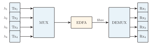
Wavelength-division multiplexing system.

System Capabilities and Constraints

• Capacity scaling: Aggregate capacity is approximately the sum of the channel rates, so adding usable wavelengths increases fibre capacity without laying another cable.

• Independent channels: Each wavelength may carry a different client protocol or data rate, such as Ethernet, SDH/SONET, or storage-area-network traffic, within the capabilities of its transponder and optical path.

• Physical limits: Channel count and transmission reach are constrained by wavelength spacing, filter selectivity, amplifier noise, chromatic dispersion, nonlinear optical effects, and optical-component cost.

Technology Variations: CWDM and DWDM

Feature	CWDM	DWDM
Full form	Coarse Wavelength-Division Multiplexing	Dense Wavelength-Division Multiplexing
Channel spacing	Wide, typically $20\,\mathrm{nm}$	Narrow, commonly $100\,\mathrm{GHz}$ (about $0.8\,\mathrm{nm}$ near $1550\,\mathrm{nm}$) or less
Channel count	Fewer wavelengths	Many wavelengths
Laser requirement	Simpler, often uncooled lasers	Precise, temperature-controlled lasers
Typical use	Shorter metro and access links	High-capacity metro-core and long-haul backbone links

WDM System Components

Component	Function
Optical transmitter	Generates a modulated optical carrier at a specific, stable wavelength
Optical multiplexer	Combines several wavelengths onto a single optical fibre
EDFA (Erbium-Doped Fibre Amplifier)	Amplifies multiple WDM channels directly in the optical domain without optical-electrical-optical conversion
Optical demultiplexer	Separates the received composite signal into its individual wavelengths
OADM (Optical Add-Drop Multiplexer)	Adds or removes selected wavelengths at an intermediate node while allowing others to pass through
ROADM (Reconfigurable Optical Add-Drop Multiplexer)	Uses remote software control to reconfigure which wavelengths are added, dropped, or switched

Comparison of Multiplexing Techniques

Feature / criterion	Space-Division Multiplexing (SDM)	Frequency-Division Multiplexing (FDM)	Time-Division Multiplexing (TDM)	Wavelength-Division Multiplexing (WDM)
Fundamental concept	Allocates a distinct physical path or spatial channel to each signal.	Divides the available bandwidth into non-overlapping frequency channels.	Allocates the shared link to different signals sequentially in recurring time slots.	Carries several optical channels on one fibre using different light wavelengths $\lambda$.
Separation basis	Physical conductors, fibre cores, spatial modes, or antenna paths.	Carrier-frequency bands in the electrical or radio spectrum.	Interleaved time slots grouped into frames.	Optical wavelengths or corresponding optical frequencies.
Domain of operation	Spatial or physical dimension.	Frequency domain.	Time domain.	Optical spectrum.
Core mechanism	Uses separate pairs/fibres, multi-core or few-mode fibre, or spatial streams separated by MIMO processing.	Modulators translate signals to assigned carriers; a linear combiner forms the composite signal and filters separate the channels.	Electronic switches or commutators interleave samples, bits, or bytes; framing identifies each recurring slot.	Optical filters, diffraction gratings, thin-film filters, or arrayed waveguide gratings (AWGs) combine and separate wavelengths.
Signal type	Carries analog or digital signals.	Carries analog signals or digitally modulated carrier signals.	Predominantly digital; sampled analog signals can also be multiplexed before quantisation in analog TDM systems.	Optical carriers whose modulated payloads may use different protocols and bit rates.
Capacity constraints	Number of available paths, physical size, antenna count, and spatial crosstalk or mode coupling.	Total usable bandwidth, channel bandwidths, guard bands, filter selectivity, noise, and link SNR.	Aggregate line rate, switching and clock speed, framing overhead, and sampling rate when analog inputs are digitised.	Usable optical bands, channel spacing, chromatic and polarisation-mode dispersion, fibre nonlinearities, and optical-amplifier bandwidth.
Overhead and efficiency	Low multiplexing overhead but high hardware overhead from additional conductors, cores, or antennas.	Guard bands reduce spectral efficiency but limit adjacent-channel interference.	Frame-alignment bits and, where required, guard time reduce payload efficiency; fixed synchronous slots are wasted when idle.	Channel spacing and filter roll-off consume optical spectrum; tighter grids require more precise components.
Synchronisation need	Separate physical paths need no multiplexing synchronisation; coherent MIMO implementations require aligned signal processing.	No common frame clock; receivers require carrier tuning, and coherent modulation also requires phase or frequency recovery.	Accurate clock and frame synchronisation is essential to prevent bit slips and slot misalignment.	No common time-slot clock at the WDM layer, but laser wavelength stability requires precise frequency and temperature control.
Real-world examples	Multi-pair telephone cables; $4\times4$ or $8\times8$ MIMO in 5G/Wi-Fi; multi-core fibre.	AM/FM radio; analog cable TV; ADSL subcarriers.	T1/E1 carrier systems; ISDN; GSM time slots.	CWDM metro/access links; DWDM terrestrial and submarine long-haul networks.
Primary engineering challenge	Deployment cost, physical scaling limits, and crosstalk between spatial paths.	Adjacent-channel interference, intermodulation, and the need for selective filters and linear equipment.	Clock recovery, jitter, frame alignment, and increasing aggregate line rate as more channels are added.	Precision-laser and filter cost, dispersion and nonlinearities, and accumulated optical-amplifier noise over long spans.

Core Metrics

1. FDM and WDM operating domains: WDM follows the frequency-separation principle of FDM, but their implementations differ. FDM normally operates from kilohertz to gigahertz using electronic oscillators, mixers, and electrical filters. WDM operates in the photonic domain at hundreds of terahertz, commonly near $1550\,\mathrm{nm}$; for example, $193.1\,\mathrm{THz}$ corresponds to approximately $1552.5\,\mathrm{nm}$. It uses wavelength-selective devices such as thin-film filters, diffraction gratings, and AWGs, while EDFAs amplify light through stimulated emission from erbium ions.

2. PCM-TDM synchronisation: In T1 and E1 systems, each voice channel contributes one PCM sample to every frame. Since telephony PCM uses an $8\,\mathrm{kHz}$ sampling rate,

$$f_{\text{frame}}=8000\ \text{frames/s},\qquad T_{\text{frame}}=\frac{1}{f_{\text{frame}}}=125\,\mu\mathrm{s}.$$

The receiver recovers the line clock and frame alignment to locate each user’s slot. Excessive uncorrected clock drift or jitter can produce bit slips or loss of frame alignment and consequently corrupt multiple tributary channels.

1. WDM nonlinearities: Closely spaced DWDM channels at high optical power can alter the refractive index of the fibre through the Kerr effect.

• Four-wave mixing (FWM): Interacting optical channels generate new frequencies such as $f_i+f_j-f_k$; a product that falls inside another channel causes interference.

• Self-phase modulation (SPM): A channel’s own intensity changes its phase, producing chirp and spectral broadening.

• Cross-phase modulation (XPM): Power variations in one channel change the phase of neighbouring channels, increasing distortion.

Multiplexing vs Multiple Access

• Multiplexing: Combines tributary signals within a transmission system, for example several PCM channels at one trunk multiplexer.

• Multiple access: Coordinates separate users sharing a common resource, for example mobile stations assigned uplink time slots or subcarriers. It must account for users’ timing, power, and access requests as well as channel separation.

Multiple access	Based on	Example
FDMA	Frequency	1G cellular, satellite
TDMA	Time slot	GSM
CDMA	Code	IS-95, CDMA2000
OFDMA	Orthogonal subcarriers	LTE, WiMAX, 5G NR
SDMA	Space / beam	Sector antennas, MIMO

Common multiple-access methods

TeleTraffic Engineering

Note

Teletraffic engineering

is the application of traffic theory, probability, and statistical mechanics to the design, planning, dimensioning, and performance optimization of telecommunication networks. It aims to cost-effectively balance network capacity (resources like trunks, bandwidth, and switches) against the dynamic, unpredictable demand of users to achieve a specified Quality of Service (QoS).

Importance of Teletraffic Engineering

• Models stochastic demand: User traffic varies randomly with time, so probability-based models are needed to estimate busy-hour load.

• Avoids over- and under-provisioning: Excess capacity wastes capital and remains idle, while insufficient capacity causes congestion, blocking, and excessive delay.

• Balances cost and service quality: Traffic models identify the minimum practical capacity that satisfies the required Grade of Service (GoS) or Quality of Service (QoS).

Operational Metrics

Busy Hour and BHCA

The busy hour is the continuous 60-minute interval with the highest traffic demand. Busy-Hour Call Attempts (BHCA) is the total number of call setup attempts, successful or unsuccessful, made during that hour; it measures switch and signalling workload rather than circuit occupancy.

$$\lambda_{\mathrm{BH}}=\frac{\mathrm{BHCA}}{3600}\ \text{attempts/s};\qquad \text{for example, }18{,}000\ \mathrm{BHCA}=5\ \text{attempts/s}.$$

BHCA alone does not determine traffic in erlangs; the mean holding time is also required: $A=\lambda h$.

Calling Rate ($\lambda$)

The calling rate is the number of calls in a selected traffic stream during an observation interval:

$$\lambda=\frac{N}{T}\quad\text{calls per unit time}.$$

Use $\lambda_o=N_a/T$ for offered attempts and $\lambda_c=N_c/T$ for accepted calls.

Mean Holding Time ($h$)

The holding time is how long a call occupies or requests a network resource. For $N$ calls of durations $t_i$,

$$h=\frac{1}{N}\sum_{i=1}^{N}t_i.$$

The calls used to calculate $h$ must be from the same offered or carried population as $\lambda$.

Traffic Volume ($V$)

Traffic volume is the total resource-occupancy time accumulated during the observation interval:

$$V=\sum_{i=1}^{N}t_i,$$

usually expressed in circuit-minutes or circuit-hours.

Traffic Intensity ($A$) and the Erlang

Traffic intensity is the average number of resources occupied during interval $T$:

$$A=\frac{V}{T}=\lambda h\quad\text{erlangs (E)}.$$

The units of $\lambda$ and $h$ must be compatible. One erlang means that one circuit is occupied continuously on average; for example, 60 circuit-minutes during one hour equals $1\,\mathrm{E}$.

Blocking Probability ($B$)

The blocking probability is the probability that an offered call cannot obtain a resource. Its observed estimate is

$$B\approx\frac{N_b}{N_a},$$

where $N_b$ is the number of blocked attempts and $N_a$ is the total number of offered attempts.

Offered, Carried, and Lost Traffic

Offered traffic $A_o$ is total demand, carried traffic $A_c$ is successfully served demand, and lost traffic $A_l$ is blocked demand. For blocking probability $B$,

$$A_o=A_c+A_l,\qquad A_c=A_o(1-B),\qquad A_l=A_oB.$$

These relations assume blocked and accepted calls have the same mean offered holding time, as in the Erlang loss model.

Circuit Utilisation ($\rho$)

For a group of $m$ identical circuits carrying $A_c$ erlangs, the mean utilisation per circuit is

$$\rho=\frac{A_c}{m},\qquad \text{occupancy}=100\rho\%.$$

Grade of Service (GoS)

Grade of Service is a specified traffic-performance target under stated busy-hour conditions. A loss system commonly requires

$$B\leq B_{\max},$$

while a waiting system may specify a delay target such as $P\{W_q>t_0\}\leq p_{\max}$.

Erlang B Formula

The Erlang B model, or Erlang loss formula, gives the probability that an arriving call is blocked because all $m$ circuits are occupied. It represents a full-availability loss system with no waiting room, conventionally written as an $M/M/m/m$ queue.

Model Assumptions

• Poisson arrivals: Calls arrive independently at a constant mean rate $\lambda$ from a population large relative to the trunk group.

• Blocked calls cleared (BCC): A call finding all circuits busy is rejected immediately; it neither waits nor holds a place in a queue.

• Holding times: Accepted calls have independent holding times with mean $h$. The $M/M/m/m$ derivation assumes exponential holding times, although Erlang B is insensitive to their distribution under the standard loss-system assumptions.

• Full availability: Any arriving call can seize any one of the $m$ identical free circuits, and each accepted call occupies one circuit until completion.

• Steady state: Arrival and service conditions are stable, with no priorities, reservations, immediate retrials, or dependent overflow traffic.

Offered Traffic

The offered traffic intensity is

$$A=\lambda h\quad\text{erlangs},$$

where $\lambda$ is the offered call rate and $h$ is the mean holding time in compatible units. One erlang represents the continuous average occupancy of one circuit.

Blocking Probability

Note

Erlang B loss formula

$$B(A,m)=\frac{\dfrac{A^m}{m!}}{\displaystyle\sum_{k=0}^{m}\dfrac{A^k}{k!}},$$

where $A$ is the offered traffic in erlangs, $m$ is the number of circuits, and $k$ represents the possible number of occupied circuits. The result $B(A,m)$ is both the blocking probability and the loss-system Grade of Service (GoS).

The corresponding carried and lost traffic are

$$A_c=A\left[1-B(A,m)\right],\qquad A_l=A\,B(A,m).$$

Numerically Stable Recursion

For calculation, the recursive form avoids large powers and factorials:

$$B(A,0)=1,\qquad B(A,m)=\frac{A\,B(A,m-1)}{m+A\,B(A,m-1)}.$$

Trunk Dimensioning and Application

• Dimensioning: For busy-hour traffic $A$ and target GoS $B_{\max}$, choose the smallest integer $m$ satisfying $B(A,m)\leq B_{\max}$; for a $2\%$ target, $B_{\max}=0.02$.

• Capacity planning: The model balances the cost of excess circuits against the blocking caused by insufficient capacity.

• Model boundary: Erlang B predicts call blocking, not waiting time. Use a queueing model such as Erlang C when blocked calls wait instead of being cleared.

Queuing Theory

Note

Queuing theory

is the mathematical study of waiting lines used to analyze and predict performance when data packets or voice calls contend for limited network resources. It models how traffic moves through components like packet buffers, routers, and switches to optimize network delays, capacity, and packet loss.

Kendall’s Notation

Kendall’s notation is a standard method for describing and classifying a queueing model. Its complete form is

$$A/S/c/K/N/D,$$

where the service-time field $S$ is also written as $B$, giving the alternative form $A/B/c/K/N/D$.

Arrival Process ($A$)

Describes how customers arrive at the system.

• M (Markovian): Arrivals form a Poisson process; equivalently, interarrival times are independent and exponentially distributed.

• D (Deterministic): Customers arrive at fixed, regular intervals.

• G (General): Interarrival times follow a general probability distribution.

Service-Time Distribution ($S$ or $B$)

Describes the time required to serve each customer.

• M (Markovian): Service times are independent and exponentially distributed.

• D (Deterministic): Every customer has the same constant service time.

• G (General): Service times follow a general probability distribution.

Number of Parallel Servers ($c$)

The positive integer $c$ gives the number of servers operating simultaneously. For example, $c=1$ denotes one server and $c=m$ denotes $m$ parallel servers.

System Capacity ($K$)

$K$ is the maximum number of customers allowed in the entire system, including those in service and those waiting. If omitted, $K=\infty$ is normally assumed.

Calling Population ($N$)

$N$ is the number of potential customers that may generate arrivals. If omitted, $N=\infty$ is normally assumed.

Queue Discipline ($D$)

$D$ specifies the rule used to select the next waiting customer.

• FCFS/FIFO: First Come, First Served (First In, First Out).

• LCFS/LIFO: Last Come, First Served (Last In, First Out).

• SIRO: Service in Random Order.

Standard Example: $M/M/1$

The notation $M/M/1$ describes Poisson arrivals, exponential service times, and one server. Because the final fields are omitted, it conventionally means

$$M/M/1/\infty/\infty/\mathrm{FCFS}.$$

Little’s Law (Little’s Theorem)

Little’s Law states that the long-term average number of customers, calls, packets, or jobs in a stable queueing system equals their effective arrival rate multiplied by their average time in that system:

$$L=\lambda W,\qquad L_q=\lambda W_q.$$

The first relation applies to the complete system, while the second applies only to the waiting queue.

Components

• $L$: Mean number of customers, packets, or jobs in the system, including those waiting and in service.

• $\lambda$: Effective or admitted arrival rate into the system per unit time.

• $W$: Mean total time in the system, including waiting time and service time.

• $L_q$: Mean number of customers, calls, packets, or jobs waiting in the queue, excluding those currently in service.

• $W_q$: Mean waiting time before service begins.

Conditions

• The system must be stable, its long-run averages must exist, and flow must be conserved.

• Each relation must use the same customer population and observation boundary.

• If arrivals are rejected, $\lambda$ must be the admitted throughput rather than the total offered rate.

• Poisson arrivals, exponential service times, and a particular discipline such as FIFO or LIFO are not required.

Importance

• Distribution-independent: It applies to Poisson, deterministic, or general arrival and service distributions when the stated conditions hold.

• Flexible: The system and queue forms relate occupancy, throughput, and delay when analysing network buffers and server performance.

M/M/1 Queue

In Kendall’s notation, M/M/1 denotes Markovian (Poisson) arrivals, Markovian (exponential) service times, and one server. The omitted fields imply an unlimited system capacity, an infinite calling population, and FCFS service.

Let calls, packets, or jobs arrive at mean rate $\lambda$. The server completes them at mean rate $\mu$ while busy, so the mean service time is $1/\mu$. A steady state exists only when $\lambda<\mu$.

Symbols

Symbol	Meaning	Unit
$\lambda$	Mean arrival rate	Customers per unit time
$\mu$	Mean service rate while the server is busy	Customers per unit time
$\rho$	Server utilisation or traffic intensity, $\lambda/\mu$	Dimensionless
$P_n$	Probability that exactly $n$ customers are in the system	Dimensionless
$L$	Mean number in the system, including the customer in service	Customers
$L_q$	Mean number waiting in the queue	Customers
$W$	Mean total time in the system, including service	Time
$W_q$	Mean waiting time before service	Time

Performance Formulae

Utilisation and state probabilities

$$\rho=\frac{\lambda}{\mu}<1,\qquad P_0=1-\rho,\qquad P_n=(1-\rho)\rho^n.$$

Mean number of customers

$$L=\frac{\rho}{1-\rho}=\frac{\lambda}{\mu-\lambda},$$ $$L_q=\frac{\rho^2}{1-\rho} =\frac{\lambda^2}{\mu(\mu-\lambda)}.$$

Mean delay

$$W=\frac{1}{\mu-\lambda},$$ $$W_q=\frac{\lambda}{\mu(\mu-\lambda)} =\frac{\rho}{\mu-\lambda}.$$

The results satisfy Little’s Law and the service-time relation:

$$L=\lambda W,\qquad L_q=\lambda W_q,\qquad W=W_q+\frac{1}{\mu}.$$

As $\rho\to1$, $L$, $L_q$, $W$, and $W_q$ grow without bound. Increasing buffer space alone cannot correct sustained overload; the long-term service rate must remain greater than the arrival rate.

Feature	Erlang B	Queuing model
System type	Loss system	Waiting system
Blocked user	Cleared immediately	Waits in queue
Main metric	Blocking probability	Delay, queue length
Example	Trunk group (no wait)	Router buffer, call centre
Typical formula	Erlang B	Little’s law, M/M/1, M/M/c

Erlang B loss model vs. queuing (delay) model

Solved Examples

Note

Example: Traffic intensity of a subscriber

A subscriber makes 4 calls during a busy hour, with a mean holding time of 3 minutes. The total holding time is $4\times3=12$ minutes, so the traffic intensity is

$$A=\frac{12}{60}=0.2\,E.$$

[!NOTE]

Example: Erlang B blocking probability

A full-availability loss group has 4 trunks and receives 2 erlangs of Poisson offered traffic. With blocked calls cleared, its blocking probability is

$$B(2,4)=\frac{2^4/4!}{1+2+2^2/2!+2^3/3!+2^4/4!} =\frac{0.6667}{7}\approx0.0952,$$

so about $9.52\%$ of attempts are blocked. The carried traffic is $2(1-0.0952)\approx1.810$ erlangs.

[!NOTE]

Example: M/M/1 router delay

Model a router output as an M/M/1 queue with arrival rate $\lambda=80$ packets/s and service rate $\mu=100$ packets/s. Since $\lambda<\mu$, the queue has a steady state.

$$\rho=\frac{80}{100}=0.8,\quad L=\frac{0.8}{0.2}=4,\quad W=\frac{1}{100-80}=0.05\,s.$$

The server is busy $80\%$ of the time, with 4 packets in the system on average. The $50\,\mathrm{ms}$ mean system delay includes $1/\mu=10\,\mathrm{ms}$ of service, so mean queueing delay is $W_q=40\,\mathrm{ms}$ and $L_q=\lambda W_q=3.2$ packets.

[!NOTE]

Example: TDM and E1/PCM-30 frame (10 marks)

• TDM: Interleaves tributary words in time. Synchronous TDM gives each source a fixed recurring slot; statistical TDM assigns capacity to active sources and uses identifiers and buffers. The receiver needs synchronisation to separate channels correctly.

• PCM voice: Speech limited to about $3.4\,\mathrm{kHz}$ is sampled at $8\,\mathrm{kHz}$. With 8 bits per sample, each channel produces $8000\times8=64\,\mathrm{kbit/s}$.

• E1 frame: Contains 32 eight-bit slots every $125\,\mu\mathrm{s}$, giving

$$32\times8=256\ bit,\quad f_{\text{frame}}=\frac{1}{125\,\mu\text{s}}=8000\ \text{fr/s},$$$$R_{\text{E1}}=256\times8000=2.048\,Mbit/s.$$

• PCM-30 slot allocation:

  • TS1–TS15 and TS17–TS31 carry 30 bearer channels, with payload rate $30\times64=1.920\,\mathrm{Mbit/s}$.

  • TS0 carries frame alignment and related overhead. TS16 carries channel-associated signalling across a 16-frame multiframe; other E1 service configurations can use a different signalling arrangement.

• T1/DS1: Carries 24 eight-bit channel words plus one framing bit per $125\,\mu\mathrm{s}$. Its frame size is $24\times8+1=193$ bits and line rate is $193\times8000=1.544\,\mathrm{Mbit/s}$.

• Trade-off: Recurring PCM slots give deterministic rates and support digital switching, but idle slots cannot be reassigned without a different multiplexing scheme. Loss of frame alignment can disrupt many channels simultaneously.

[!NOTE]

Example: Traffic intensity and Erlang B (5 marks)

• Traffic intensity: $A=\lambda h$ erlangs, where arrival rate and mean holding time use compatible units. One erlang is one circuit’s average occupancy; one 60-minute call or thirty 2-minute calls during an hour each represent one erlang of traffic.

• Offered and carried load: For blocking probability $B$, carried traffic is $A_c=A_o(1-B)$ and lost traffic is $A_l=A_oB$. A loss-system GoS commonly specifies a maximum busy-hour blocking probability.

• Erlang B model: Independent Poisson calls occupy one of $m$ identical, fully accessible trunks. Calls finding all trunks busy are cleared, without waiting. Holding times are independent with a specified mean; exponential times give the elementary derivation, though the result is insensitive to their distribution under these assumptions.

$$B(A,m)=\frac{A^m/m!}{\sum_{k=0}^{m}A^k/k!},\qquad B(A,0)=1,\ B(A,m)=\frac{A\,B(A,m-1)}{m+A\,B(A,m-1)}.$$

For $A=2$ erlangs and $m=4$, blocking is $9.52\%$, which fails a $1\%$ GoS target. More trunks are needed. Erlang B does not predict queue delay; correlated retrials, strongly bursty arrivals, or a small finite source population require a different model.

[!NOTE]

Example: Queuing theory and grade of service (5 marks)

• Queue model: Arrivals wait when the server is busy, provided waiting space is available. Arrival statistics, service times, server count, buffer capacity, source population, and service discipline determine waiting and loss behavior.

• Kendall notation: $A/S/c/K/N/D$ specifies those properties. M/M/1 denotes Poisson arrivals, exponential service times, one server, and conventionally an unlimited FIFO queue with an effectively infinite source population.

• Grade of service: A loss system is often specified by blocking probability. A waiting system can be specified by mean delay or the probability that waiting exceeds a limit, $P\{W_q>t\}$.

• Little’s law: $L=\lambda W$ and $L_q=\lambda W_q$ relate mean occupancy to admitted throughput and mean time for the same stable system. Queue-only measures exclude service time.

• M/M/1 results: For $\rho=\lambda/\mu<1$, $L=\rho/(1-\rho)$ and $W=1/(\mu-\lambda)$. With $\lambda=80\,\mathrm{s^{-1}}$ and $\mu=100\,\mathrm{s^{-1}}$, utilisation is $0.8$, mean occupancy is 4, and mean system time is $0.05\,\mathrm{s}$.

• Capacity constraint: Delay rises without bound as utilisation approaches 1 in this model. A finite delay target therefore requires service capacity above the long-run arrival rate, not merely a larger buffer.