Magnetostatics and Maxwell’s Equations

Note

Magnetostatics.

Magnetostatics is the study of magnetic fields produced by steady currents, for which charge density and current density do not vary with time.

Current and Current Density

Note

Electric current and current density.

Electric current $I$ is charge flow rate, while current density $\mathbf J$ specifies current flow per unit cross-sectional area and direction.

$$I=\frac{dq}{dt}.$$ $$I=\int_S\mathbf{J}\cdot d\mathbf{S}.$$

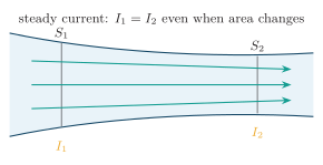
Current continuity in a tapered conducting tube.

Note

Conduction current density.

Conduction current density is the physical drift current per unit area in a conducting material; for a linear isotropic conductor it obeys the point form of Ohm’s law, $\mathbf J=\sigma\mathbf E$.

$$\mathbf{J}=\sigma\mathbf{E}.$$

In a dielectric, charges do not cross the material in the same way, but a time-varying electric flux density can still act as a current term in Maxwell’s equations.

Magnetic Fields

Note

Magnetic flux density and magnetic field intensity.

Magnetic flux density $\mathbf B$ measures magnetic flux per unit normal area, while magnetic field intensity $\mathbf H$ describes the magnetizing field produced by free current; a linear medium relates them through $\mathbf B=\mu\mathbf H$.

$$\mathbf{B}=\mu\mathbf{H}.$$

$\mu$ is the absolute permeability of the medium. $\mathbf{B}$ is measured in tesla, and $\mathbf{H}$ is measured in amperes per metre.

Biot-Savart Law

Note

Biot-Savart law.

The Biot-Savart law gives the magnetic field contribution produced by each steady current element; its direction follows $d\mathbf l\times\mathbf a_R$ and its magnitude decreases with distance squared.

For a steady current element,

$$d\mathbf{H}=\frac{I\,d\mathbf{l}\times\mathbf{a}_R}{4\pi R^2}.$$

The field $\mathbf{H}$ is determined by current geometry; the material response enters later through $\mathbf{B}=\mu\mathbf{H}$.

For a complete current path,

$$\mathbf{H}=\int_C\frac{I\,d\mathbf{l}\times\mathbf{a}_R}{4\pi R^2}.$$

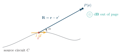
Source-to-observation geometry for the Biot-Savart law.

Applying this geometry to a finite straight segment converts the path integral into angular end limits.

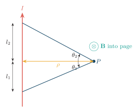
Field geometry of a finite straight current segment.

Closing the current path into a circular loop makes all transverse field contributions cancel on the axis.

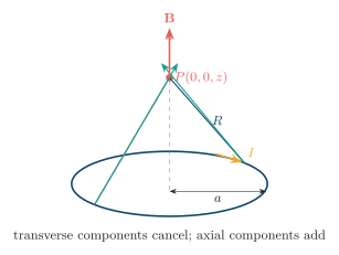
Biot-Savart construction for the field on a circular loop axis.

Infinite Straight Conductor

Let a current $I$ flow in the $+z$-direction. At radial distance $\rho$,

$$d\mathbf l=dz'\mathbf a_z, \qquad \mathbf R=\rho\mathbf a_\rho-z'\mathbf a_z, \qquad d\mathbf l\times\mathbf R=\rho\,dz'\mathbf a_\phi.$$

The Biot-Savart integral becomes

$$\begin{aligned} \mathbf H & =\frac{I\rho}{4\pi}\mathbf a_\phi \int_{-\infty}^{\infty}\frac{dz'}{(\rho^2+z'^2)^{3/2}} \\ & =\boxed{\frac{I}{2\pi\rho}\mathbf a_\phi}. \end{aligned}$$

Thus $\mathbf B=\mu I\mathbf a_\phi/(2\pi\rho)$. The field forms concentric circles whose direction follows the right-hand grip rule.

Circular Loop at Its Centre

For a circular loop of radius $a$, every current element is perpendicular to its displacement vector toward the centre, is the same distance $a$ away, and produces a field in the same axial direction. Therefore

$$H=\oint_C\frac{I\,dl}{4\pi a^2} =\frac{I}{4\pi a^2}(2\pi a) =\boxed{\frac{I}{2a}}.$$

For a closely wound $N$-turn coil,

$$\boxed{\mathbf H=\frac{NI}{2a}\mathbf a_n}, \qquad \boxed{\mathbf B=\frac{\mu NI}{2a}\mathbf a_n},$$

where $\mathbf a_n$ is set by the current direction and the right-hand rule.

Standard results:

Current geometry	Magnetic field
Infinite straight wire	$H_\phi=\dfrac{I}{2\pi\rho}$
Circular loop, centre	$H=\dfrac{I}{2a}$
Long solenoid	$H=nI$
Toroid	$H_\phi=\dfrac{NI}{2\pi\rho}$

Ampere’s Circuital Law

Note

Ampere’s circuital law.

In magnetostatics, the circulation of magnetic field intensity around a closed path equals the steady conduction current enclosed by that path.

Integral form for steady current:

$$\oint_C\mathbf{H}\cdot d\mathbf{l}=I_{\text{enc}}.$$

The left side measures circulation of magnetic field intensity around the closed contour $C$. The right side is the current passing through any surface bounded by that contour.

Differential form:

$$\nabla\times\mathbf{H}=\mathbf{J}.$$

This steady-current form is exact for magnetostatics. Time-varying fields require an additional displacement-current term, introduced below, so that current remains continuous through regions such as capacitor gaps.

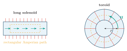
Amperian paths for a long solenoid and a toroid.

Within a uniformly current-filled conductor, the enclosed current grows with the area of the chosen Amperian circle.

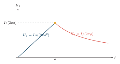
Magnetic field intensity of a solid conductor with uniform current density.

For a solid conductor of radius $a$ carrying uniformly distributed current $I$, a circular path of radius $\rho<a$ encloses $I\rho^2/a^2$. Consequently,

$$\mathbf H(\rho)= \begin{cases} \dfrac{I\rho}{2\pi a^2}\mathbf a_\phi, & 0\le\rho<a, \\[0.7em] \dfrac{I}{2\pi\rho}\mathbf a_\phi, & \rho\ge a. \end{cases}$$

For a long solenoid having $N$ turns over length $l$, let $n=N/l$. A rectangular Amperian path of axial length $L$ links $nL$ turns. Neglecting the external and end fields gives

$$HL=nLI, \qquad \boxed{\mathbf H=nI\mathbf a_z}, \qquad \boxed{\mathbf B=\mu nI\mathbf a_z}.$$

For an ideal toroid with $N$ turns, a circular path inside the core links all turns:

$$H_\phi(2\pi\rho)=NI, \qquad \boxed{\mathbf H=\frac{NI}{2\pi\rho}\mathbf a_\phi}.$$

The ideal external field is approximately zero because a path outside the toroid encloses zero net turn current.

Ampere’s law is most useful when symmetry makes $\mathbf{H}$ constant along an Amperian path.

Biot-Savart and Ampere Methods

Feature	Biot-Savart law	Ampere’s circuital law
Method	sums source-element fields	relates circulation to linked current
Required geometry	arbitrary, if integrable	high symmetry for direct solution
Field direction	from the cross product	inferred from symmetry
Best suited to	finite wires, arcs and loops	infinite wires, solenoids and toroids
Time domain	steady-current form	Maxwell form includes displacement current

Biot-Savart integration is the more general direct calculation. Ampere’s law is faster when a path can be chosen on which $\mathbf H$ is tangential and constant.

Curl in Magnetostatics

Note

Curl in magnetostatics.

Curl measures local circulation; in magnetostatics, conduction current density is the source of magnetic-field circulation, $\nabla\times\mathbf H=\mathbf J$.

Thus,

$$\mathbf{J}=\nabla\times\mathbf{H}.$$

Magnetic flux has no isolated source or sink:

$$\nabla\cdot\mathbf{B}=0.$$

Magnetic Scalar and Vector Potential

Note

Magnetic potential.

A magnetic potential is an auxiliary scalar or vector field from which the physical magnetic field can be recovered by differentiation.

Magnetic scalar potential. In a simply connected current-free region, magnetic scalar potential $V_m$ is defined by $\mathbf H=-\nabla V_m$; for a uniform medium it satisfies $\nabla^2V_m=0$.

In a simply connected region with no free current,

$$\nabla\times\mathbf{H}=0.$$

Hence $\mathbf{H}$ can be written as the negative gradient of a magnetic scalar potential $V_m$:

$$\mathbf{H}=-\nabla V_m.$$

For a uniform medium with no current in the region, $\nabla\cdot\mathbf{B}=0$ and $\mathbf{B}=\mu\mathbf{H}$ give

$$\nabla^2V_m=0.$$

The scalar magnetic potential is not generally single-valued around paths that enclose current.

Note

Magnetic vector potential.

Magnetic vector potential $\mathbf A$ is a vector field defined by $\mathbf B=\nabla\times\mathbf A$; it is not unique because adding the gradient of any scalar function leaves $\mathbf B$ unchanged.

Since the divergence of a curl is always zero and $\nabla\cdot\mathbf{B}=0$, a magnetic vector potential $\mathbf{A}$ may always be defined by

$$\mathbf{B}=\nabla\times\mathbf{A}.$$

For a linear medium,

$$\mathbf{H}=\frac{1}{\mu}\nabla\times\mathbf{A}.$$

The vector potential is not unique, because adding the gradient of any scalar function to $\mathbf{A}$ leaves $\nabla\times\mathbf{A}$ unchanged. With the common Coulomb gauge $\nabla\cdot\mathbf{A}=0$ and uniform $\mu$, magnetostatics gives

$$\nabla^2\mathbf{A}=-\mu\mathbf{J}.$$

For a localized current distribution, the corresponding Green-function solution is

$$\boxed{\mathbf A(\mathbf r)=\frac{\mu}{4\pi} \int_V\frac{\mathbf J(\mathbf r')}{\lvert\mathbf r-\mathbf r'\rvert}\,dV'}.$$

For a thin filament carrying current $I$, this reduces to

$$\boxed{\mathbf A(\mathbf r)=\frac{\mu I}{4\pi} \int_C\frac{d\mathbf l'}{\lvert\mathbf r-\mathbf r'\rvert}}.$$

The two potential descriptions have different domains of usefulness:

Feature	Scalar potential $V_m$	Vector potential $\mathbf A$
Field relation	$\mathbf H=-\nabla V_m$	$\mathbf B=\nabla\times\mathbf A$
Valid region	current-free and simply connected	general magnetostatic field
Uniform-medium equation	$\nabla^2V_m=0$	$\nabla^2\mathbf A=-\mu\mathbf J$
Typical use	gaps and magnetic circuits	current distributions, flux and inductance
Nonuniqueness	may be multivalued around current	has gauge freedom

$$\Phi=\int_S\mathbf{B}\cdot d\mathbf{S} =\oint_C\mathbf{A}\cdot d\mathbf{l}.$$

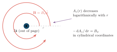
Magnetic vector potential around a line current.

Faraday’s Law of Induction

Note

Faraday’s law of induction.

Faraday’s law states that changing magnetic flux through a circuit produces an electromotive force equal to the negative time rate of change of flux linkage.

For a single-turn stationary loop,

$$e=-\frac{d\Phi}{dt}, \qquad \Phi=\int_S\mathbf{B}\cdot d\mathbf{S}.$$

Note

Lenz’s law.

The induced emf drives current in the direction whose magnetic effect opposes the change in flux that produced it; this opposition is represented by the minus sign in Faraday’s law.

For an $N$-turn coil with the same flux linking each turn,

$$e=-N\frac{d\Phi}{dt}.$$

For a fixed loop, the induced emf is also the circulation of electric field intensity around the boundary curve $C$:

$$\oint_C\mathbf{E}\cdot d\mathbf{l} =-\frac{d}{dt}\int_S\mathbf{B}\cdot d\mathbf{S} =-\int_S\frac{\partial\mathbf{B}}{\partial t}\cdot d\mathbf{S}.$$

Using Stokes’ theorem gives the local differential form

$$\nabla\times\mathbf{E}=-\frac{\partial\mathbf{B}}{\partial t}.$$

Thus a time-varying magnetic field produces a circulating electric field, even when no conducting wire is present.

Maxwell’s Equations

Note

Maxwell’s equations.

Maxwell’s equations are the four fundamental field laws relating electric charge, magnetic flux, electromagnetic induction, conduction current and displacement current. Differential forms describe local behavior; integral forms describe net behavior over finite paths, surfaces or volumes.

Maxwell’s equations are fundamental laws based on experiment; they are not derived from one another. The following steps derive the differential form of each law from its corresponding integral form.

Gauss’s Law for Electricity

Start with the integral law over a closed surface $\partial V$:

$$\oint_{\partial V}\mathbf{D}\cdot d\mathbf{S} =Q_{\text{enc}} =\int_V\rho_v\,dV.$$

Apply the divergence theorem to the flux integral:

$$\oint_{\partial V}\mathbf{D}\cdot d\mathbf{S} =\int_V\nabla\cdot\mathbf{D}\,dV.$$

Equating the two volume integrals gives

$$\int_V\left(\nabla\cdot\mathbf{D}-\rho_v\right)dV=0.$$

Because this is true for every arbitrary volume $V$, the integrand must vanish at every point. Therefore,

$$\boxed{\nabla\cdot\mathbf{D}=\rho_v}.$$

Gauss’s Law for Magnetism

There are no observed isolated magnetic charges, so the net magnetic flux through any closed surface is zero:

$$\oint_{\partial V}\mathbf{B}\cdot d\mathbf{S}=0.$$

Apply the divergence theorem:

$$\int_V\nabla\cdot\mathbf{B}\,dV=0.$$

Since this holds for every arbitrary volume $V$,

$$\boxed{\nabla\cdot\mathbf{B}=0}.$$

This means magnetic field lines form closed loops rather than beginning or ending at magnetic monopoles.

Faraday’s Law of Electromagnetic Induction

For a fixed contour $C=\partial S$, Faraday’s integral law is

$$\oint_C\mathbf{E}\cdot d\mathbf{l} =-\frac{d}{dt}\int_S\mathbf{B}\cdot d\mathbf{S}.$$

Because the surface is fixed, move the time derivative inside the integral:

$$-\frac{d}{dt}\int_S\mathbf{B}\cdot d\mathbf{S} =-\int_S\frac{\partial\mathbf{B}}{\partial t}\cdot d\mathbf{S}.$$

Apply Stokes’ theorem to the line integral:

$$\oint_C\mathbf{E}\cdot d\mathbf{l} =\int_S(\nabla\times\mathbf{E})\cdot d\mathbf{S}.$$

Equating the surface integrals gives

$$\int_S\left( \nabla\times\mathbf{E}+\frac{\partial\mathbf{B}}{\partial t} \right)\cdot d\mathbf{S}=0.$$

Since this is true for every arbitrary surface $S$,

$$\boxed{ \nabla\times\mathbf{E}=-\frac{\partial\mathbf{B}}{\partial t} }.$$

Ampere-Maxwell Law

The magnetostatic equation $\nabla\times\mathbf{H}=\mathbf{J}$ cannot by itself describe time-varying charge. Taking its divergence would give

$$\nabla\cdot(\nabla\times\mathbf{H}) =\nabla\cdot\mathbf{J} \quad\Longrightarrow\quad 0=\nabla\cdot\mathbf{J}.$$

However, conservation of charge requires

$$\nabla\cdot\mathbf{J}=-\frac{\partial\rho_v}{\partial t}.$$

Differentiate Gauss’s law $\nabla\cdot\mathbf{D}=\rho_v$ with respect to time:

$$\nabla\cdot\frac{\partial\mathbf{D}}{\partial t} =\frac{\partial\rho_v}{\partial t}.$$

Adding this relation to the continuity equation gives

$$\nabla\cdot\left( \mathbf{J}+\frac{\partial\mathbf{D}}{\partial t} \right)=0.$$

Thus the displacement-current density $\mathbf{J}_d=\partial\mathbf{D}/\partial t$ completes the current source in time-varying fields. The corrected integral law is

$$\oint_C\mathbf{H}\cdot d\mathbf{l} =\int_S\left( \mathbf{J}+\frac{\partial\mathbf{D}}{\partial t} \right)\cdot d\mathbf{S}.$$

Apply Stokes’ theorem to the left-hand side:

$$\int_S(\nabla\times\mathbf{H})\cdot d\mathbf{S} =\int_S\left( \mathbf{J}+\frac{\partial\mathbf{D}}{\partial t} \right)\cdot d\mathbf{S}.$$

Because this holds for every arbitrary surface $S$,

$$\boxed{ \nabla\times\mathbf{H} =\mathbf{J}+\frac{\partial\mathbf{D}}{\partial t} }.$$

Summary

Law	Differential form	Integral form
Gauss law for electricity	$\nabla\cdot\mathbf{D}=\rho_v$	$\oint_S\mathbf{D}\cdot d\mathbf{S}=Q_{\text{enc}}$
Gauss law for magnetism	$\nabla\cdot\mathbf{B}=0$	$\oint_S\mathbf{B}\cdot d\mathbf{S}=0$
Faraday law	$\nabla\times\mathbf{E}=-\dfrac{\partial\mathbf{B}}{\partial t}$	$\oint_C\mathbf{E}\cdot d\mathbf{l}=-\dfrac{d}{dt}\int_S\mathbf{B}\cdot d\mathbf{S}$
Ampere-Maxwell law	$\nabla\times\mathbf{H}=\mathbf{J}+\dfrac{\partial\mathbf{D}}{\partial t}$	$\oint_C\mathbf{H}\cdot d\mathbf{l}=I_c+\dfrac{d}{dt}\int_S\mathbf{D}\cdot d\mathbf{S}$

Interpretation of each equation:

Equation	Physical meaning
Gauss law for electricity	Electric flux leaving a closed surface equals the charge enclosed by that surface.
Gauss law for magnetism	Net magnetic flux through any closed surface is zero; magnetic field lines do not begin or end on isolated magnetic charges.
Faraday law	Changing magnetic flux produces circulating electric field.
Ampere-Maxwell law	Conduction current and changing electric flux both produce circulating magnetic field.

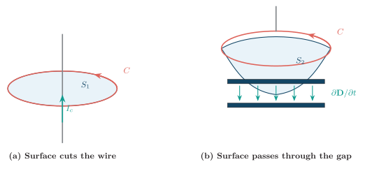
Capacitor surfaces for Maxwell equation integral forms.

Displacement Current

Note

Displacement current density.

Displacement current density $\mathbf J_d$ is the time rate of change of electric flux density; it produces magnetic-field circulation even where no conduction charge crosses the medium.

Thus,

$$\mathbf{J}_d=\frac{\partial\mathbf{D}}{\partial t}$$

A charging capacitor is the standard example. In the wires, current is conduction current. Across the dielectric gap, charge does not physically cross from plate to plate, but $\mathbf{D}=\varepsilon\mathbf{E}$ changes with time as the plate charge and voltage change. The term $\partial\mathbf{D}/\partial t$ completes Ampere’s law through the capacitor gap and makes the same enclosed-current result independent of which surface spans the loop.

The total current density used in the Ampere-Maxwell law is therefore

$$\mathbf{J}_{\text{total}}=\mathbf{J}+\mathbf{J}_d =\sigma\mathbf{E}+\frac{\partial\mathbf{D}}{\partial t}.$$

Charge Continuity

Note

Charge-continuity equation.

The charge-continuity equation is the local statement of charge conservation: net current flowing out of a volume equals the rate at which charge inside decreases.

Its differential form is

$$\nabla\cdot\mathbf{J}=-\frac{\partial\rho_v}{\partial t}.$$

This relation is consistent with the Ampere-Maxwell law and Gauss’s law.

Field Boundary Conditions

Note

Electromagnetic boundary conditions.

At an interface, normal $\mathbf D$ changes by free surface charge density, normal $\mathbf B$ is continuous, tangential $\mathbf E$ is continuous, and tangential $\mathbf H$ changes by surface current density.

Consider two materials separated by an interface. Let $\mathbf a_{n12}$ be the unit normal directed from medium 1 to medium 2. The boundary conditions describe the behavior of the four principal static field vectors $\mathbf E$, $\mathbf D$, $\mathbf H$ and $\mathbf B$ across that interface.

Boundary Conditions for $\mathbf E$ and $\mathbf D$

Two independent conditions apply at a dielectric interface.

First, the tangential component of electric field intensity is continuous:

$$\mathbf a_{n12}\times(\mathbf E_2-\mathbf E_1)=0, \qquad E_{t1}=E_{t2}.$$

Since $\mathbf D=\varepsilon_0\varepsilon_r\mathbf E$, the corresponding tangential flux-density components satisfy

$$\frac{D_{t1}}{\varepsilon_{r1}} =\frac{D_{t2}}{\varepsilon_{r2}}.$$

Second, the normal component of electric flux density has a discontinuity equal to the free surface charge density $\rho_s$ (also written $\sigma_s$):

$$\mathbf a_{n12}\cdot(\mathbf D_2-\mathbf D_1)=\rho_s,$$

or, in scalar normal components,

$$D_{n2}-D_{n1}=\rho_s, \qquad \varepsilon_{r2}E_{n2}-\varepsilon_{r1}E_{n1} =\frac{\rho_s}{\varepsilon_0}.$$

Equivalently, $D_{n1}-D_{n2}=-\rho_s$. Reversing the chosen unit normal reverses the signs in the scalar jump equation, but not the physical boundary condition.

For the usual charge-free dielectric interface, $\rho_s=0$, so

$$D_{n1}=D_{n2}, \qquad \varepsilon_{r1}E_{n1}=\varepsilon_{r2}E_{n2}.$$

If $\theta_1$ and $\theta_2$ are the angles made by $\mathbf E_1$ and $\mathbf E_2$ with the interface itself, then $\tan\theta_i=E_{ni}/E_{ti}$. Combining normal-$\mathbf D$ continuity with tangential-$\mathbf E$ continuity gives the electric-field refraction law

$$\boxed{\frac{\tan\theta_1}{\tan\theta_2} =\frac{\varepsilon_{r2}}{\varepsilon_{r1}}} \qquad (\rho_s=0).$$

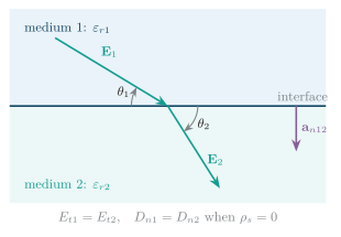
Electric-field refraction at a charge-free dielectric interface.

Boundary Conditions for $\mathbf H$ and $\mathbf B$

Let the two materials have conductivities $\sigma_1$, $\sigma_2$ and relative permeabilities $\mu_{r1}$, $\mu_{r2}$.

Because magnetic monopoles do not exist, the normal component of magnetic flux density is continuous:

$$\mathbf a_{n12}\cdot(\mathbf B_2-\mathbf B_1)=0, \qquad B_{n1}=B_{n2}.$$

Either orientation may be chosen for the unit normal; the same scalar equality results.

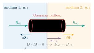
A Gaussian pillbox across a magnetic interface.

At a current-free interface, the tangential component of magnetic field strength is continuous:

$$\mathbf a_{n12}\times(\mathbf H_2-\mathbf H_1)=0, \qquad H_{t1}=H_{t2}.$$

For angles $\theta_1$ and $\theta_2$ measured from the interface, continuity of $B_n$ gives $\mu_{r1}H_{n1}=\mu_{r2}H_{n2}$. Together with $H_{t1}=H_{t2}$, this gives the magnetic-field refraction law

$$\boxed{\frac{\tan\theta_1}{\tan\theta_2} =\frac{\mu_{r2}}{\mu_{r1}}} \qquad (\mathbf K_s=0).$$

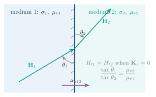
Magnetic-field refraction at a current-free interface.

If a free surface-current sheet exists at the interface, the tangential component of $\mathbf H$ is discontinuous. Its vector boundary condition is

$$\boxed{\mathbf a_{n12}\times(\mathbf H_2-\mathbf H_1)=\mathbf K_s},$$

which can equivalently be written in the form

$$(\mathbf H_1-\mathbf H_2)\times\mathbf a_{n12}=\mathbf K_s.$$

Here $\mathbf K_s$ (also written $\mathbf K$ or $\mathbf K_0$) is the free surface-current density in $\mathrm{A/m}$, and the magnitude of the tangential jump is $\lvert\mathbf K_s\rvert$. Conducting materials can support such a sheet current, but nonzero bulk conductivity alone does not determine $\mathbf K_s$; the jump is produced by the actual surface current.

The four general boundary conditions are therefore

$$\mathbf a_{n12}\cdot(\mathbf D_2-\mathbf D_1)=\rho_s, \qquad \mathbf a_{n12}\cdot(\mathbf B_2-\mathbf B_1)=0,$$ $$\mathbf a_{n12}\times(\mathbf E_2-\mathbf E_1)=0, \qquad \mathbf a_{n12}\times(\mathbf H_2-\mathbf H_1)=\mathbf K_s.$$

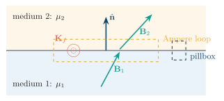
Pillbox and loop constructions at a magnetic boundary.

The same pillbox and loop constructions yield the general normal and tangential electromagnetic boundary conditions.

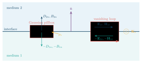
Interface constructions for electromagnetic boundary conditions.

At a perfect electric conductor, those general conditions reduce to zero tangential electric field at the surface.

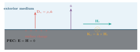
Perfect electric conductor boundary conditions.