DFT, IDFT, and the FFT

Discrete Fourier Transform

The discrete Fourier transform (DFT) converts a finite-length discrete-time sequence into a finite set of equally spaced frequency samples. For an $N$-point sequence $x[n]$,

Caution

Key Formula — The $N$-point DFT

$$X[k]=\sum_{n=0}^{N-1}x[n]e^{-\mathrm{j}2\pi kn/N}, \qquad k=0,1,\ldots,N-1.$$

The DFT treats the listed samples as one period of a sequence that repeats with period $N$. This periodic-extension assumption is what later makes multiplication of DFTs correspond to circular rather than ordinary linear convolution.

Meaning of the Frequency Index

If the time samples were obtained at sampling frequency $F_s$, adjacent DFT bins are separated by

Caution

Key Formula — DFT-bin spacing

$$\Delta f=\frac{F_s}{N}.$$

Equivalently, bin $k$ samples normalized angular frequency

$$\Omega_k=\frac{2\pi k}{N}\quad(\operatorname{mod}2\pi), \qquad f_k=\frac{kF_s}{N}\quad(\operatorname{mod}F_s).$$

Discrete-time frequency is periodic with period $F_s$, so the upper DFT bins represent negative frequencies. In signed-frequency order,

Caution

Key Formula — Signed frequency represented by bin $k$

$$f_k= \begin{cases} \dfrac{kF_s}{N}, & 0\leq k\leq\left\lfloor N/2\right\rfloor, \\[6pt] \dfrac{(k-N)F_s}{N}, & \left\lfloor N/2\right\rfloor<k\leq N-1. \end{cases}$$

Thus $k=0$ is DC, the lower nonzero bins represent positive frequencies, and the upper bins wrap around to negative frequencies. For even $N$, bin $k=N/2$ is the Nyquist-frequency bin at $F_s/2$, equivalently $-F_s/2$; those two endpoints denote the same discrete-time frequency.

A centred or fftshift display merely rearranges the bins so that negative frequencies appear before DC and positive frequencies; it changes neither their values nor their physical interpretation. Also distinguish the grid spacing $F_s/N$ from resolving power: the former is set by transform length, whereas separation of nearby tones is governed by the nonzero record duration and its window.

Twiddle Factor and Matrix View

Define the $N$th-root-of-unity, or twiddle, factor

Caution

Key Formula — DFT twiddle factor

$$W_N=e^{-\mathrm{j}2\pi/N}, \qquad X[k]=\sum_{n=0}^{N-1}x[n]W_N^{kn}.$$

The transform can then be written as the matrix product

Caution

Key Formula — DFT matrix

$$\begin{bmatrix} X[0] \\ X[1]\\ X[2]\\ \vdots\\ X[N-1] \end{bmatrix} = \begin{bmatrix} 1 & 1 & 1 & \cdots & 1 \\ 1 & W_N & W_N^2 & \cdots & W_N^{N-1} \\ 1 & W_N^2 & W_N^4 & \cdots & W_N^{2(N-1)} \\ \vdots & \vdots & \vdots & \ddots & \vdots \\ 1 & W_N^{N-1} & W_N^{2(N-1)} & \cdots & W_N^{(N-1)^2} \end{bmatrix} \begin{bmatrix} x[0] \\ x[1]\\ x[2]\\ \vdots\\ x[N-1] \end{bmatrix}.$$

The rows of the DFT matrix are sampled complex sinusoids. Each row correlates the input samples with one frequency bin.

Let $\mathbf{F}_N=[W_N^{kn}]_{k,n=0}^{N-1}$. Distinct basis sinusoids are orthogonal because

Caution

Key Formula — Roots-of-unity orthogonality

$$\sum_{n=0}^{N-1}W_N^{(k-r)n} = \begin{cases} N, & k\equiv r\pmod N, \\ 0, & k\not\equiv r\pmod N. \end{cases}$$$$\mathbf{F}_N^{\mathsf H}\mathbf{F}_N=N\mathbf{I}, \qquad \mathbf{F}_N^{-1}=\frac{1}{N}\mathbf{F}_N^{\mathsf H}.$$

Thus the rows and columns have norm $\sqrt{N}$ and are mutually orthogonal. The normalized matrix $\mathbf{F}_N/\sqrt{N}$ is unitary. This identity both explains the IDFT and supplies the short proof of Parseval’s theorem in the section.

Inverse Discrete Fourier Transform

The inverse DFT (IDFT) reconstructs the time-domain samples from the DFT coefficients:

Caution

Key Formula — The $N$-point IDFT

$$x[n]=\frac{1}{N}\sum_{k=0}^{N-1}X[k]e^{\mathrm{j}2\pi kn/N}, \qquad n=0,1,\ldots,N-1.$$

The forward and inverse equations form the transform pair

$$x[n]\ \longleftrightarrow\ X[k].$$

They differ in the sign of the exponential and in the factor $1/N$ assigned to the inverse transform.

Important DFT Properties

Let $(q)_N$ mean $q$ reduced modulo $N$, and suppose $x[n]\longleftrightarrow X[k]$.

1. Linearity: For constants $a$ and $b$,

$$ax_1[n]+bx_2[n] \longleftrightarrow aX_1[k]+bX_2[k].$$

The spectrum of a weighted sum is the same weighted sum of the individual spectra.

2. Periodicity: The frequency-domain sequence obeys

$$X[k+N]=X[k].$$

Both the finite time sequence and its DFT are treated as one period of periodic sequences.

3. Circular time shift: A shift by $n_0$ samples changes only spectral phase:

$$x[(n-n_0)_N] \longleftrightarrow e^{-\mathrm{j}2\pi kn_0/N}X[k].$$

4. Frequency shift: Multiplication by a DFT-bin complex exponential shifts the spectrum circularly by $k_0$ bins:

$$x[n]e^{\mathrm{j}2\pi k_0n/N} \longleftrightarrow X[(k-k_0)_N].$$

5. Circular convolution: For an $N$-point circular convolution,

$$x[n]\circledast_N h[n] \longleftrightarrow X[k]H[k].$$

This identity is the basis of fast convolution using the DFT or FFT.

6. Conjugate symmetry: If $x[n]$ is real, then

$$X[(-k)_N]=X^*[k].$$

Consequently, the negative-frequency half is the complex conjugate of the positive-frequency half.

For a real input, $X[0]$ is real and, when $N$ is even, $X[N/2]$ is also real. Hence only $\lfloor N/2\rfloor+1$ bins are independent. Magnitude is circularly even and phase is circularly odd wherever the spectrum is nonzero. A real circularly even sequence has a real DFT; a real circularly odd sequence has a purely imaginary DFT, with zero DC and zero Nyquist value when the latter bin exists.

Complete DFT Examples

Note

Example — Four-Point DFT of a Constant Sequence

Find the four-point DFT of $x[n]=\{1,1,1,1\}$. Direct substitution gives

$$X[k]=\sum_{n=0}^{3}e^{-\mathrm{j}2\pi kn/4}.$$

For $k=0$,

$$X[0]=1+1+1+1=4.$$

For $k=1,2,3$, the four roots of unity in the corresponding sum cancel, so

$$\boxed{X[k]=\{4,0,0,0\}}.$$

The constant sequence therefore contains only a DC component.

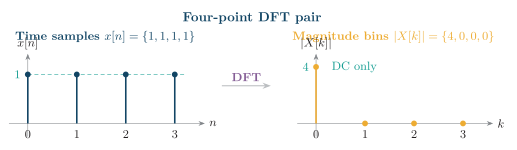
DFT pair for a constant four-sample sequence. Equal time samples produce a single nonzero DC coefficient; all nonzero-frequency roots of unity cancel.

Note

Example — Four-Point DFT of a Nonconstant Sequence

For $x[0]=1$, $x[1]=2$, $x[2]=3$, and $x[3]=4$, use $W_4=e^{-\mathrm{j}2\pi/4}=-\mathrm{j}$ in

$$X[k]=\sum_{n=0}^{3}x[n]W_4^{kn}.$$

The four coefficients are

$$\begin{aligned} X[0] & =1+2+3+4=10, \\ X[1] & =1+2(-\mathrm{j})+3(-1)+4(\mathrm{j})=-2+\mathrm{j}2, \\ X[2] & =1+2(-1)+3(1)+4(-1)=-2, \\ X[3] & =X^*[1]=-2-\mathrm{j}2. \end{aligned}$$

Hence

$$\boxed{X[k]=\{10,-2+\mathrm{j}2,-2,-2-\mathrm{j}2\}}.$$

The conjugate pair $X[1]$ and $X[3]$ confirms the expected symmetry for a real input sequence.

Fast Fourier Transform

The fast Fourier transform (FFT) is an efficient algorithm for computing a DFT. It is not a different transform: its output is the same $X[k]$ defined by the DFT equation, obtained by exploiting root-of-unity symmetries and repeated smaller transforms.

Method	Complex multiplications	Complexity
Direct DFT	approximately $N^2$	$O(N^2)$
Radix-2 FFT	approximately $\dfrac{N}{2}\log_2N$	$O(N\log_2N)$

Direct DFT and radix-2 FFT computational costs.

For large $N$, the reduction from quadratic to nearly linear-logarithmic growth is substantial.

Radix-2 Decimation Derivation

When $N$ is a power of two, divide the input into its even- and odd-indexed samples,

$$x_e[r]=x[2r], \qquad x_o[r]=x[2r+1], \qquad 0\leq r<N/2.$$

Let $E[k]$ and $O[k]$ be the $N/2$-point DFTs of these two subsequences. Splitting the original DFT sum yields

$$\begin{aligned} X[k] & =\sum_{r=0}^{N/2-1}x[2r]W_N^{2rk} +\sum_{r=0}^{N/2-1}x[2r+1]W_N^{(2r+1)k} \\ & =\sum_{r=0}^{N/2-1}x[2r]W_{N/2}^{rk} +W_N^k\sum_{r=0}^{N/2-1}x[2r+1]W_{N/2}^{rk} \\ & =E[k]+W_N^kO[k]. \end{aligned}$$

Because $E[k]$ and $O[k]$ are periodic with period $N/2$ and $W_N^{k+N/2}=-W_N^k$, the second half of the transform is available from the same pair of smaller DFTs:

Caution

Key Formula — Radix-2 combine equations

$$\begin{aligned} X[k] & =E[k]+W_N^kO[k], \\ X[k+N/2] & =E[k]-W_N^kO[k], \qquad 0\leq k<N/2. \end{aligned}$$

These sum-and-difference equations form one radix-2 butterfly.

Two common radix-2 organizations are decimation in time (DIT), which recursively splits the input samples, and decimation in frequency (DIF), which recursively splits the output-frequency bins. Both compute the same DFT and use the same basic butterfly arithmetic.

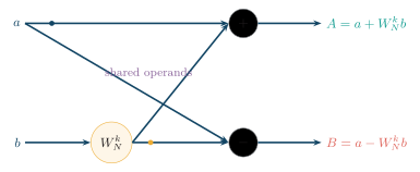
Radix-2 butterfly. One twiddle multiplication and a shared sum–difference pair produce two DFT outputs.

Each butterfly performs one complex multiplication by a twiddle factor, one addition, and one subtraction. A radix-2 FFT has $\log_2N$ stages and $N/2$ butterflies per stage, giving approximately

Caution

Key Formula — Radix-2 operation counts

$$\frac{N}{2}\log_2N\ \text{complex multiplications}, \qquad N\log_2N\ \text{complex additions}.$$

This replaces the approximately $N^2$ operations needed by direct DFT evaluation.

In a common in-place DIT implementation, the inputs are arranged in bit-reversed order and the outputs emerge in natural order. Bit reversal is an implementation arrangement, not a requirement of every FFT program; other memory layouts and DIF implementations place the permutation elsewhere.

For the four-point flow graph, reversing the two binary index bits gives

Natural index	Binary index	Reversed index
$0$	$00$	$0$
$1$	$01$	$2$
$2$	$10$	$1$
$3$	$11$	$3$

so natural order $0,1,2,3$ becomes the input order $0,2,1,3$. In general, an $N=2^M$ radix-2 transform reverses $M$ binary index bits.

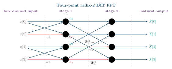
Two-stage four-point decimation-in-time FFT. Bit-reversed inputs $x(0),x(2),x(1),x(3)$ pass through two butterflies per stage and produce $X(0),\ldots,X(3)$ in natural order.

Spectral Leakage and Windowing

The DFT sees only a finite observation. If a conceptually longer sequence $x_\infty[n]$ is observed through a length-$L$ window $w[n]$, the analysed record is

$$x_r[n]=x_\infty[n]w[n].$$

Time-domain multiplication convolves the original spectrum with the window spectrum. For the rectangular window $w[n]=1$, $0\leq n<L$, its DTFT is

Caution

Key Formula — Rectangular-window spectrum

$$W_r(e^{\mathrm{j}\Omega}) =e^{-\mathrm{j}\Omega(L-1)/2} \frac{\sin(L\Omega/2)}{\sin(\Omega/2)},$$

with limiting value $L$ at $\Omega=0$. The main lobe and sidelobes of this Dirichlet kernel spread a sinusoid into neighbouring DFT bins whenever its frequency is not exactly on the DFT grid. This spreading is spectral leakage; it is not frequency aliasing.

• Coherent record: A bin-centred sinusoid completes an integer number of cycles in the record. With a rectangular window, its ideal spectrum falls on the corresponding conjugate bin pair.

• Tapered windows: Hann, Hamming, and Blackman windows suppress sidelobes and help expose a weak tone near a strong one.

• Resolution trade-off: Sidelobe suppression widens the main lobe. A window cannot simultaneously give the narrowest main lobe and the lowest leakage; a longer nonzero record is needed for better physical resolution.

• Amplitude and noise scaling: A window changes tone amplitude and equivalent noise bandwidth. Correct a coherent tone by $G_c=L^{-1}\sum_{n=0}^{L-1}w[n]$, while PSD normalization depends on $\sum_n|w[n]|^2$.

Zero Padding and Frequency Resolution

Appending zeros to the $L$ measured samples and taking an $N_z$-point DFT, $N_z>L$, samples the same windowed-record DTFT on the denser grid $F_s/N_z$. This produces a smoother spectrum, facilitates peak interpolation, permits an efficient FFT length, and supplies the length needed for linear convolution.

Tip

Exam Focus — What zero padding cannot do

Zero padding adds calculated frequency samples, not observed time samples. It does not add information, remove leakage, narrow the window’s main lobe, or make two physically unresolved tones resolvable. Only extending the nonzero observation can improve that underlying resolution.

Applications and Quick Review

FFT computation is central to spectrum analysis, OFDM communication systems, fast convolution, and audio and image processing.

Tip

Exam Focus — DFT and FFT Quick Review

• The DFT maps $N$ finite samples to $N$ equally spaced frequency bins; the IDFT reconstructs the samples from those coefficients, and $\Delta f=F_s/N$.

• The DFT basis is orthogonal: $\mathbf{F}_N^{\mathsf H}\mathbf{F}_N=N\mathbf{I}$. For real data, $X[(-k)_N]=X^*[k]$.

• An FFT computes that same DFT while reducing complexity from $O(N^2)$ to $O(N\log_2N)$.

• DFT-domain multiplication gives $N$-point circular convolution, not unqualified linear convolution.

• Windowing controls the main-lobe–sidelobe trade-off. Zero padding interpolates the sampled spectrum but does not create resolution.