Signals, Classification, and Standard Signals

What a Signal Represents

A signal is a function that carries information about the state or behaviour of a physical system. Its independent variable is often time, but it can also be distance, frequency, temperature, or another measurable quantity. Signal classification is not mere terminology: it determines which energy measure, transform, sampling rule, and system test is appropriate.

Continuous, Discrete, Analog, and Digital Signals

• Continuous-time (CT) signal $x(t)$: Defined for every real value of $t$.

• Discrete-time (DT) signal $x[n]$: Defined only at integer indices $n$; sampling a CT signal gives $x[n]=x(nT_s)$.

• Analog signal: Has a continuous amplitude range, whether its independent variable is continuous or sampled.

• Digital signal: Has discrete time and a finite, quantized set of amplitude values.

Discrete time does not by itself mean digital: the sample values of $x[n]$ may still have continuous precision until quantization is applied.

Periodic and Aperiodic Signals

Caution

Key Formula — Periodicity tests

$$x(t+T_0)=x(t)\quad\text{(CT)}, \qquad x[n+N_0]=x[n]\quad\text{(DT)}.$$

The smallest positive $T_0$ or positive integer $N_0$ satisfying the relevant identity is the fundamental period. A signal with no such value is aperiodic. The CT sinusoid $A\cos(\omega_0t+\phi)$ has $T_0=2\pi/|\omega_0|$. A DT sinusoid $A\cos(\Omega_0n+\phi)$ is periodic only if $\Omega_0/(2\pi)$ is rational; if $\Omega_0/(2\pi)=p/q$ in lowest terms, the fundamental period of a nonconstant sinusoid is $N_0=q$, equivalently the least positive integer satisfying $\Omega_0N_0=2\pi k$. A nonzero constant signal is periodic, but because every positive shift is a period in CT, it has no unique fundamental CT period.

Even and Odd Decomposition

An even signal satisfies $x(-t)=x(t)$, while an odd signal satisfies $x(-t)=-x(t)$. Typical even signals are $\cos t$ and $|t|$; typical odd signals are $\sin t$ and $t$. Every signal has the unique decomposition

Caution

Key Formula — Even and odd components

$$x(t)=x_e(t)+x_o(t),\qquad x_e(t)=\frac{x(t)+x(-t)}{2},\qquad x_o(t)=\frac{x(t)-x(-t)}{2}.$$

The same identities hold with $t$ replaced by $n$. Symmetry often halves a transform calculation: real even signals have real even spectra, and real odd signals have imaginary odd spectra.

Deterministic, Random, and Support Classes

A deterministic signal is specified exactly, for example $A\cos\omega_ct$. A random or stochastic signal is described statistically through quantities such as mean, variance, probability density, and autocorrelation. Noise and practical message waveforms are commonly modelled as random processes.

With respect to support, a causal signal is zero for $t<0$, an anti-causal signal is zero for $t>0$, and a two-sided signal is nonzero on both sides of the origin. The DT definitions replace $t$ by $n$. These signal labels must not be confused with system causality, which states that an output cannot depend on future input values.

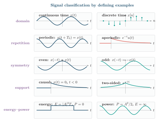
Native examples of the principal signal classifications. Each trace satisfies the definition printed in its panel; a signal can belong to several classes simultaneously.

Tip

Exam Focus

Classifications are independent. For example, $e^{-t}u(t)$ is continuous-time, aperiodic, deterministic, causal, and an energy signal. State every applicable property and justify it using the defining equation.

Compact Method for Time Operations

For

Caution

Key Formula — Amplitude and time operations

$$y(t)=A\,x\!\left(a(t-t_0)\right),$$

$A$ scales the amplitude, $t_0$ shifts the result to the right, $a<0$ reverses time, and $|a|>1$ compresses the time axis. The safest construction is to map each recognizable feature: a feature of $x(t)$ at $t=\tau$ appears in $y(t)$ where

$$a(t-t_0)=\tau \quad\Longrightarrow\quad t=t_0+\frac{\tau}{a}.$$

For example, $x(t)=u(t+1)-u(t-2)$ is a unit pulse on $-1\leq t<2$. In $y(t)=x(2t+4)$, its edges move to $t=-5/2$ and $t=-1$, so the pulse is compressed by two and lies on $-5/2\leq t<-1$. Solving for feature locations avoids the common error of applying a shift and a scale in the wrong order.

Energy and Average Power

Energy measures total squared magnitude, whereas average power measures its long-term time average. For complex signals the magnitude square is $|x|^2=x x^*$.

Caution

Key Formula — Continuous- and discrete-time definitions

$$\begin{aligned} E_x^{\mathrm{CT}} &=\int_{-\infty}^{\infty}|x(t)|^2\,\mathrm{d}t, & P_x^{\mathrm{CT}} &=\lim_{T\to\infty}\frac{1}{2T} \int_{-T}^{T}|x(t)|^2\,\mathrm{d}t,\\ E_x^{\mathrm{DT}} &=\sum_{n=-\infty}^{\infty}|x[n]|^2, & P_x^{\mathrm{DT}} &=\lim_{N\to\infty}\frac{1}{2N+1} \sum_{n=-N}^{N}|x[n]|^2. \end{aligned}$$

The power limits are understood only when they exist. An energy signal has $0<E_x<\infty$; dividing its bounded accumulated energy by an indefinitely long observation interval gives $P_x=0$. A power signal has $0<P_x<\infty$; its accumulated energy must then grow without bound, so $E_x=\infty$.

Class	Total energy	Average power	Typical example
Energy signal	$0<E_x<\infty$	$P_x=0$	Square-integrable finite pulse or decaying transient
Power signal	$E_x=\infty$	$0<P_x<\infty$	Nonzero sinusoid or periodic square wave
Neither	Fails $0<E_x<\infty$	Fails $0<P_x<\infty$	$x(t)=t$, for which both measures diverge

Energy and power signal comparison.

No nonzero signal can satisfy both strict class definitions. The zero signal has $E_x=P_x=0$ and is normally placed in neither class because both definitions require a positive measure. A finite-duration signal is an energy signal only when it is square-integrable; finite duration by itself does not license an infinite-amplitude waveform. Likewise, “nondecaying” alone does not guarantee finite average power. A nonzero periodic signal is a power signal when its squared magnitude has a finite, positive integral (or sum) over one period.

Note

Example — Energy and Power Classification

(a) Finite CT pulse. Let

$$x(t)= \begin{cases} A, & |t|\leq T_p/2,\\ 0, & \text{otherwise}. \end{cases}$$

Then

$$E_x=\int_{-T_p/2}^{T_p/2}|A|^2\,\mathrm{d}t=|A|^2T_p, \qquad P_x=0,$$

so a nonzero finite pulse is an energy signal.

(b) CT sinusoid. For real $A$ and $\omega_0\neq0$, average over one period $T_0$:

$$P_x=\frac{1}{T_0}\int_0^{T_0} A^2\cos^2(\omega_0t+\phi)\,\mathrm{d}t =\frac{A^2}{2}, \qquad E_x=\infty.$$

Thus the sinusoid is a power signal.

(c) Decaying DT sequence. For $x[n]=C a^n u[n]$ with $|a|<1$,

$$E_x=|C|^2\sum_{n=0}^{\infty}|a|^{2n} =\frac{|C|^2}{1-|a|^2}, \qquad P_x=0.$$

It is a DT energy signal. By contrast, $C e^{\mathrm{j}\Omega_0n}$ has $P_x=|C|^2$ and $E_x=\infty$ for $C\neq0$.

Standard Signals

The unit impulse $\delta(t)$, unit step $u(t)$, ramp $r(t)$, signum $\operatorname{sgn}(t)$, and normalized sinc $\operatorname{sinc}(t)=\sin(\pi t)/(\pi t)$ form a compact vocabulary for constructing and analysing more complicated signals.

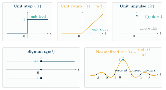
Normalized elementary continuous-time signals. The impulse arrow denotes unit area, not a finite height; the normalized sinc has $\operatorname{sinc}(0)=1$ and zeros at every nonzero integer.

the figure uses an arrow for the impulse because its area, rather than a finite plotted height, is the meaningful quantity. Unless stated otherwise, this section uses the angular-frequency Fourier convention

Caution

Key Formula — Angular-frequency Fourier convention

$$X(\omega)=\int_{-\infty}^{\infty}x(t)e^{-\mathrm{j}\omega t}\,\mathrm{d}t, \qquad x(t)=\frac{1}{2\pi}\int_{-\infty}^{\infty} X(\omega)e^{\mathrm{j}\omega t}\,\mathrm{d}\omega.$$

Unit Step Function

The continuous-time unit step is

Caution

Key Formula — Unit step

$$u(t)= \begin{cases} 0, & t<0,\\ 1, & t>0. \end{cases}$$

Its value at the single point $t=0$ is convention-dependent: common choices are $0$, $1/2$, and $1$. That choice does not affect ordinary CT integrals, but it should be stated when a point value matters. In DT the usual definition is $u[n]=1$ for $n\geq0$ and $0$ otherwise, so $u[0]=1$.

The step models a switching action or the start of a causal waveform. A shifted step $u(t-t_0)$ switches on at $t=t_0$, and $x(t)u(t-t_0)$ suppresses $x(t)$ before that instant. Under the convention above, its Fourier transform is a distribution:

Caution

Key Formula — Unit-step transform

$$u(t)\ \overset{\mathcal F}{\longleftrightarrow}\ \pi\delta(\omega) +\operatorname{PV}\!\left(\frac{1}{\mathrm{j}\omega}\right).$$

Here $\operatorname{PV}$ is the Cauchy principal-value distribution. It is essential because $1/\omega$ is singular at $\omega=0$; the formula is not an ordinary pointwise equality.

Unit Ramp Function

The unit ramp is

Caution

Key Formula — Unit ramp

$$r(t)=t\,u(t)= \begin{cases} t, & t\geq0,\\ 0, & t<0. \end{cases}$$

It models a constant-rate sweep or linearly rising input. Ramp, step, and impulse form the accumulation–differentiation chain

Caution

Key Formula — Ramp–step–impulse chain

$$r(t)=\int_{-\infty}^{t}u(\tau)\,\mathrm{d}\tau, \qquad u(t)=\frac{\mathrm{d}r(t)}{\mathrm{d}t}, \qquad \delta(t)=\frac{\mathrm{d}u(t)}{\mathrm{d}t}=\frac{\mathrm{d}^2 r(t)}{\mathrm{d}t^2}.$$

The derivative identities are distribution identities at the discontinuity. The DT ramp is commonly defined as $r[n]=n u[n]$; first differences replace derivatives in discrete time.

Signum Function

The signum function is

Caution

Key Formula — Signum

$$\operatorname{sgn}(t)= \begin{cases} -1, & t<0,\\ 0, & t=0,\\ 1, & t>0. \end{cases}$$

It represents bipolar switching and symmetric discontinuities. For $t\neq0$, $\operatorname{sgn}(t)=2u(t)-1$; the equality also holds at the origin when the symmetric choice $u(0)=1/2$ is used. Since $1\overset{\mathcal F}{\longleftrightarrow}2\pi\delta(\omega)$, cancellation of the delta terms gives, in the distribution sense,

Caution

Key Formula — Signum transform

$$\operatorname{sgn}(t)\ \overset{\mathcal F}{\longleftrightarrow}\ 2\operatorname{PV}\!\left(\frac{1}{\mathrm{j}\omega}\right).$$

This pair is also useful in Hilbert-transform derivations.

Normalized Sinc Function

This text uses the normalized definition

Caution

Key Formula — Normalized sinc

$$\operatorname{sinc}(t)= \begin{cases} \dfrac{\sin(\pi t)}{\pi t}, & t\neq0,\\[4pt] 1, & t=0, \end{cases}$$

where the value at the origin is the continuous limiting value. It is real and even, has zeros at every nonzero integer, and appears in ideal low-pass filters, rectangular-pulse spectra, sampling theory, and band-limited interpolation.

Let $\operatorname{rect}(\xi)=1$ for $|\xi|<1/2$ and $0$ for $|\xi|>1/2$; its endpoint value is immaterial to the transform integral. With the normalized sinc and the angular-frequency convention stated above,

Caution

Key Formula — Normalized sinc transform pair

$$\operatorname{sinc}(t)\ \overset{\mathcal F}{\longleftrightarrow}\ \operatorname{rect}\!\left(\frac{\omega}{2\pi}\right).$$

Thus a rectangular spectrum occupying $|\omega|<\pi$ has a sinc impulse response. The unnormalized convention $\operatorname{sinc}_u(t)=\sin t/t$ instead has zeros at $t=\pm\pi,\pm2\pi,\ldots$ and a different scaling in its transform pair; the two conventions must not be mixed.

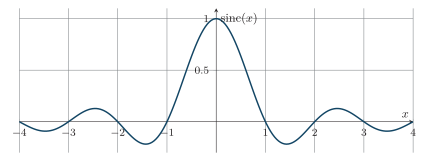
The $\operatorname{sinc}$ function — the Fourier transform of a rectangular pulse.

The sinc trace above is the frequency-domain shape obtained from a rectangular pulse. In the general pair, narrowing a rectangular pulse in one domain broadens its sinc in the other domain.

Real and Complex Exponential Signals

A real exponential has the form

$$x(t)=C e^{at},\qquad C,a\in\mathbb R.$$

It grows for $a>0$, is constant for $a=0$, and decays as $t$ increases for $a<0$. A particularly important causal transient is $e^{-at}u(t)$ with $a>0$; it is square-integrable and obeys

$$e^{-at}u(t)\ \overset{\mathcal F}{\longleftrightarrow}\ \frac{1}{a+\mathrm{j}\omega}.$$

A general complex exponential can be written

$$x(t)=C e^{st}=C e^{\sigma t}e^{\mathrm{j}\omega_0t}, \qquad s=\sigma+\mathrm{j}\omega_0.$$

The factor $e^{\sigma t}$ sets the envelope and $e^{\mathrm{j}\omega_0t}$ sets the oscillation. Euler’s identity gives the sinusoidal components

Caution

Key Formula — Euler identity

$$e^{\mathrm{j}\omega_0t}=\cos(\omega_0t)+\mathrm{j}\sin(\omega_0t).$$

Complex exponentials are eigenfunctions of LTI systems whenever the indicated response exists:

$$e^{\mathrm{j}\omega_0t}\longmapsto H(\mathrm{j}\omega_0)e^{\mathrm{j}\omega_0t}, \qquad e^{\mathrm{j}\Omega_0n}\longmapsto H(e^{\mathrm{j}\Omega_0})e^{\mathrm{j}\Omega_0n}.$$

The system changes only complex amplitude, not waveform. This is why complex exponentials form the natural basis of Fourier, Laplace, and Z-transform analysis. The DT counterparts are $C r^n$ and $C e^{\mathrm{j}\Omega_0n}$; DT frequencies separated by $2\pi k$ describe the same sequence.

Continuous-Time Unit Impulse

Interpretation as a Distribution

The Dirac delta $\delta(t)$ is not an ordinary function with a finite value at each instant. It is a generalized function, or distribution, supported at $t=0$ and defined by its action under integration:

Caution

Key Formula — Defining impulse conditions

$$\delta(t)=0\quad(t\neq0), \qquad \int_{-\infty}^{\infty}\delta(t)\,\mathrm{d}t=1.$$

The familiar “infinite height and zero width” description is only a visualization. For example, the unit-area rectangular family

$$\delta_{\Delta}(t) =\frac{1}{\Delta}\operatorname{rect}\!\left(\frac{t}{\Delta}\right), \qquad \Delta>0,$$

approaches $\delta(t)$ as $\Delta\to0^+$ in the distribution sense: for every suitable smooth test function $\varphi$,

$$\lim_{\Delta\to0^+}\int_{-\infty}^{\infty} \varphi(t)\delta_{\Delta}(t)\,\mathrm{d}t=\varphi(0).$$

It does not converge to an ordinary finite-valued function pointwise at the origin.

Nine Fundamental Properties

All products, derivatives, and transforms involving $\delta$ below are understood as distribution identities, with the ordinary factor sufficiently smooth at the impulse location.

1. Unit area and shifting: The shifted impulse is supported at $t=t_0$ and retains unit area:

$$\int_{-\infty}^{\infty}\delta(t-t_0)\,\mathrm{d}t=1.$$

An integral over an interval is one when $t_0$ lies in its interior and zero when the interval excludes $t_0$. An impulse exactly at an integration endpoint requires the adopted endpoint convention. The weighted impulse $A\delta(t-t_0)$ has strength, or area, $A$.

2. Sifting or sampling: If $x(t)$ is continuous at $t_0$, the impulse extracts its value there:

Caution

Key Formula — Continuous-time sifting

$$\int_{-\infty}^{\infty}x(t)\delta(t-t_0)\,\mathrm{d}t=x(t_0), \qquad \int_{-\infty}^{\infty}A x(t)\delta(t-t_0)\,\mathrm{d}t=A x(t_0).$$

All values away from $t_0$ make no contribution, while the unit area leaves the sampled value.

1. Multiplication identity: The corresponding distribution identity is

$$x(t)\delta(t-t_0)=x(t_0)\delta(t-t_0).$$

It means that both sides act identically on every test function; it is not a license to manipulate $\delta(0)$ as an ordinary number.

2. Time scaling: For every real $a\neq 0$,

Caution

Key Formula — Impulse scaling

$$\delta(at)=\frac{1}{|a|}\delta(t), \qquad \delta(at-b)=\frac{1}{|a|} \delta\!\left(t-\frac{b}{a}\right).$$

The reciprocal magnitude preserves the distribution’s action under a change of variable; the absolute value ensures that time reversal does not create a negative area. More generally, if the simple zeros of $g(t)$ are $t_k$, then

$$\delta(g(t))=\sum_k\frac{\delta(t-t_k)}{|g'(t_k)|}.$$

1. Even symmetry: Taking $a=-1$ in the scaling law gives

$$\delta(-t)=\delta(t).$$

Time reversal changes neither the location nor the unit area, so the impulse is even.

2. Relation to the unit step: The generalized derivative and accumulation relations are

Caution

Key Formula — Step–impulse relation

$$\delta(t)=\frac{\mathrm{d}u(t)}{\mathrm{d}t}, \qquad u(t)=\int_{-\infty}^{t}\delta(\tau)\,\mathrm{d}\tau.$$

More generally, a jump of magnitude $A$ at $t=t_0$ contributes $A\delta(t-t_0)$ to a signal’s distributional derivative.

1. Derivative of an impulse: For differentiable $x(t)$, integration by parts yields

Caution

Key Formula — Derivative sifting

$$\int_{-\infty}^{\infty}x(t)\delta'(t-t_0)\,\mathrm{d}t=-x'(t_0).$$

The sign is negative because the distributional derivative transfers the derivative to the test function. More generally,

$$\int x(t)\delta^{(m)}(t-t_0)\,\mathrm{d}t =(-1)^m x^{(m)}(t_0).$$

1. Identity under convolution: The impulse is the identity element of CT convolution, and a shifted impulse produces a matching shift:

Caution

Key Formula — Impulse convolution

$$x(t)*\delta(t)=x(t), \qquad x(t)*\delta(t-t_0)=x(t-t_0).$$

Indeed,

$$\begin{aligned} x(t)*\delta(t-t_0) &=\int_{-\infty}^{\infty} x(\tau)\delta(t-t_0-\tau)\,\mathrm{d}\tau\\ &=x(t-t_0). \end{aligned}$$

Equivalently, every suitable CT signal is a continuous superposition of shifted impulses:

$$x(t)=\int_{-\infty}^{\infty} x(\tau)\delta(t-\tau)\,\mathrm{d}\tau.$$

1. Fourier- and Laplace-transform properties: Sifting the transform kernels gives

Caution

Key Formula — Impulse transforms

$$\mathcal{F}\!\left\{\delta(t)\right\}=1, \qquad \mathcal{F}\!\left\{\delta(t-t_0)\right\}=e^{-\mathrm{j}\omega t_0},$$$$\mathcal{L}\!\left\{\delta(t)\right\}=1, \qquad \mathcal{L}\!\left\{\delta(t-t_0)\right\}=e^{-s t_0}.$$

The Laplace statements use the bilateral transform, or the common unilateral convention whose lower limit includes an impulse at the origin from $0^-$. A unit impulse has a flat Fourier spectrum and therefore excites all frequencies equally in the idealized sense.

Note

Example — Combined Scaling and Sifting

Evaluate

$$I=\int_{-\infty}^{\infty}(3t^2+2)\delta(2t-4)\,\mathrm{d}t.$$

First put the impulse in standard shifted form:

$$\delta(2t-4)=\delta\!\left(2(t-2)\right) =\frac12\delta(t-2).$$

Sifting now gives

$$I=\frac12\left[3(2)^2+2\right] =\frac{14}{2} =\boxed{7}.$$

[!NOTE]

Law — Impulse pitfalls and units

• Do not omit the absolute value in $\delta(at)=\delta(t)/|a|$.

• $\delta(t-t_0)$ is located at $t=+t_0$, not at $-t_0$.

• Apply sifting only when the impulse location lies within the stated integration interval; treat an endpoint according to the adopted convention.

• The CT impulse is defined by area and action under integration, not by a finite height. Since $\delta^2(t)$ is not defined in ordinary distribution theory, do not classify an ideal CT impulse using the usual energy integral $\int|\delta(t)|^2\,\mathrm{d}t$.

• If $t$ is measured in seconds, $\delta(t)$ has units $/s$ so that $\int\delta(t)\,\mathrm{d}t$ is dimensionless. To make $A\delta(t-t_0)$ have the units of a signal, $A$ must have units of signal-amplitude times seconds.

Discrete-Time Unit Impulse

Unlike the CT impulse, the discrete unit impulse, or unit sample, is an ordinary sequence:

Caution

Key Formula — Discrete unit impulse

$$\delta[n]= \begin{cases} 1, & n=0,\\ 0, & n\neq0. \end{cases}$$

A shift $\delta[n-n_0]$ moves the sole nonzero sample to $n=n_0$. Therefore

$$\sum_{n=-\infty}^{\infty}\delta[n-n_0]=1, \qquad \sum_{n=-\infty}^{\infty}x[n]\delta[n-n_0]=x[n_0],$$

and, equivalently,

$$x[n]\delta[n-n_0]=x[n_0]\delta[n-n_0].$$

Only the $n=n_0$ term survives. The sequence is even because $\delta[-n]=\delta[n]$, and its energy is one while its average power is zero.

The DT step relation uses a first difference rather than a derivative:

Caution

Key Formula — Discrete step–impulse relation

$$\delta[n]=u[n]-u[n-1], \qquad u[n]=\sum_{k=-\infty}^{n}\delta[k].$$

The impulse is also the identity of discrete convolution:

Caution

Key Formula — Discrete impulse convolution

$$x[n]*\delta[n]=x[n], \qquad x[n]*\delta[n-n_0]=x[n-n_0].$$

Most importantly, every DT sequence can be decomposed into scaled, shifted unit samples:

Caution

Key Formula — Unit-sample decomposition

$$\boxed{x[n]=\sum_{k=-\infty}^{\infty}x[k]\delta[n-k]}.$$

This formula is the direct bridge to convolution and the impulse-response description of an LTI system: linearity handles each weight $x[k]$, and time invariance shifts the response to each $k$.

The CT scaling rule must not be copied mechanically into DT. For example, for a nonzero integer $M$, $\delta[Mn]=\delta[n]$, not $\delta[n]/|M|$, because both sequences contain exactly one unit-valued sample at $n=0$.

Quick Review

Tip

Exam Focus — Quick Review

• Classification: Check domain, amplitude, repetition, symmetry, predictability, support, and energy or power independently.

• Energy and power: An energy signal has $0<E<\infty$ and $P=0$; a power signal has $E=\infty$ and $0<P<\infty$. A finite pulse and a nonzero sinusoid are the canonical examples.

• Even–odd split: $x_e=\tfrac 12[x(t)+x(-t)]$ and $x_o=\tfrac 12[x(t)-x(-t)]$, with identical DT formulas.

• Derivative chain: $r'(t)=u(t)$ and $u'(t)=\delta(t)$ in the distribution sense.

• Impulse rules: Sifting gives $\int x(t)\delta(t-t_0)\,\mathrm{d}t=x(t_0)$, while scaling gives $\delta(at)=\delta(t)/|a|$.

• Identity and spectrum: $x*\delta=x$ and $\mathcal{F}\!\left\{\delta(t)\right\}=1$; a shifted impulse shifts a convolution result and adds linear transform phase.

• DT synthesis: Every sequence obeys $x[n]=\sum_k x[k]\delta[n-k]$.