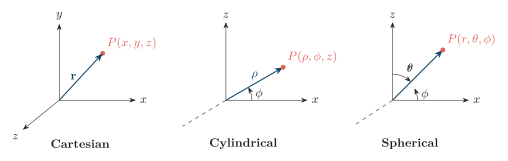
For a general vector field,
F = F x a x + F y a y + F z a z . \mathbf{F}=F_x\mathbf{a}_x+F_y\mathbf{a}_y+F_z\mathbf{a}_z. F = F x a x + F y a y + F z a z . Use the coordinate system that matches the symmetry of the source.
System Coordinates Best for Differential length Cartesian ( x , y , z ) (x,y,z) ( x , y , z ) planes, rectangular boundaries d l = d x a x + d y a y + d z a z d\mathbf{l}=dx\mathbf{a}_x+dy\mathbf{a}_y+dz\mathbf{a}_z d l = d x a x + d y a y + d z a z Cylindrical ( ρ , ϕ , z ) (\rho,\phi,z) ( ρ , ϕ , z ) lines, cylinders, coaxial structures d l = d ρ a ρ + ρ d ϕ a ϕ + d z a z d\mathbf{l}=d\rho\mathbf{a}_\rho+\rho d\phi\mathbf{a}_\phi+dz\mathbf{a}_z d l = d ρ a ρ + ρ d ϕ a ϕ + d z a z Spherical ( r , θ , ϕ ) (r,\theta,\phi) ( r , θ , ϕ ) points, spheres, radial fields d l = d r a r + r d θ a θ + r sin θ d ϕ a ϕ d\mathbf{l}=dr\mathbf{a}_r+r d\theta\mathbf{a}_\theta+r\sin\theta d\phi\mathbf{a}_\phi d l = d r a r + r d θ a θ + r sin θ d ϕ a ϕ
Coordinate systems chosen to match source symmetry.
Useful surface elements are
d S ρ = ρ d ϕ d z , d S r = r 2 sin θ d θ d ϕ . dS_\rho=\rho\,d\phi\,dz,\qquad
dS_r=r^2\sin\theta\,d\theta\,d\phi. d S ρ = ρ d ϕ d z , d S r = r 2 sin θ d θ d ϕ . Useful volume elements are
d V = d x d y d z , d V = ρ d ρ d ϕ d z , d V = r 2 sin θ d r d θ d ϕ . dV=dx\,dy\,dz,
\qquad dV=\rho\,d\rho\,d\phi\,dz,
\qquad dV=r^2\sin\theta\,dr\,d\theta\,d\phi. d V = d x d y d z , d V = ρ d ρ d ϕ d z , d V = r 2 sin θ d r d θ d ϕ . In Cartesian coordinates,
∇ = a x ∂ ∂ x + a y ∂ ∂ y + a z ∂ ∂ z . \nabla=\mathbf{a}_x\frac{\partial}{\partial x}
+\mathbf{a}_y\frac{\partial}{\partial y}
+\mathbf{a}_z\frac{\partial}{\partial z}. ∇ = a x ∂ x ∂ + a y ∂ y ∂ + a z ∂ z ∂ . ∇ V = ∂ V ∂ x a x + ∂ V ∂ y a y + ∂ V ∂ z a z . \nabla V=
\frac{\partial V}{\partial x}\mathbf{a}_x+
\frac{\partial V}{\partial y}\mathbf{a}_y+
\frac{\partial V}{\partial z}\mathbf{a}_z. ∇ V = ∂ x ∂ V a x + ∂ y ∂ V a y + ∂ z ∂ V a z . The gradient is normal to a constant- V V V
E = − ∇ V , \mathbf E=-\nabla V, E = − ∇ V , so the electric field points in the direction of the steepest decrease in potential.
∇ ⋅ F = ∂ F x ∂ x + ∂ F y ∂ y + ∂ F z ∂ z . \nabla\cdot\mathbf{F}=
\frac{\partial F_x}{\partial x}+
\frac{\partial F_y}{\partial y}+
\frac{\partial F_z}{\partial z}. ∇ ⋅ F = ∂ x ∂ F x + ∂ y ∂ F y + ∂ z ∂ F z . Equivalently, divergence is the limiting outward flux per unit volume:
∇ ⋅ F = lim Δ V → 0 1 Δ V ∮ Δ S F ⋅ d S . \nabla\cdot\mathbf F
=\lim_{\Delta V\to0}
\frac{1}{\Delta V}\oint_{\Delta S}\mathbf F\cdot d\mathbf S. ∇ ⋅ F = Δ V → 0 lim Δ V 1 ∮ Δ S F ⋅ d S . Positive divergence indicates a local source and negative divergence a local sink. In electromagnetics, ∇ ⋅ D = ρ v \nabla\cdot\mathbf D=\rho_v ∇ ⋅ D = ρ v
∇ × F = ∣ a x a y a z ∂ ∂ x ∂ ∂ y ∂ ∂ z F x F y F z ∣ . \nabla\times\mathbf{F}=
\begin{vmatrix}
\mathbf{a}_x & \mathbf{a}_y & \mathbf{a}_z \\
\frac{\partial}{\partial x} & \frac{\partial}{\partial y} & \frac{\partial}{\partial z} \\
F_x & F_y & F_z
\end{vmatrix}. ∇ × F = a x ∂ x ∂ F x a y ∂ y ∂ F y a z ∂ z ∂ F z . Equivalently,
∇ × F = ( ∂ F z ∂ y − ∂ F y ∂ z ) a x + ( ∂ F x ∂ z − ∂ F z ∂ x ) a y + ( ∂ F y ∂ x − ∂ F x ∂ y ) a z . \nabla\times\mathbf{F}=
\left(\frac{\partial F_z}{\partial y}-\frac{\partial F_y}{\partial z}\right)\mathbf{a}_x+
\left(\frac{\partial F_x}{\partial z}-\frac{\partial F_z}{\partial x}\right)\mathbf{a}_y+
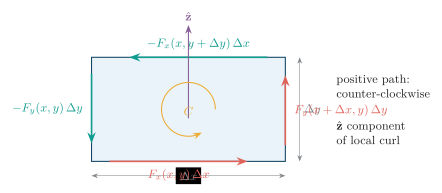
\left(\frac{\partial F_y}{\partial x}-\frac{\partial F_x}{\partial y}\right)\mathbf{a}_z. ∇ × F = ( ∂ y ∂ F z − ∂ z ∂ F y ) a x + ( ∂ z ∂ F x − ∂ x ∂ F z ) a y + ( ∂ x ∂ F y − ∂ y ∂ F x ) a z . The component normal to a small surface is the limiting circulation per unit area:
( ∇ × F ) ⋅ a n = lim Δ S → 0 1 Δ S ∮ Δ C F ⋅ d l . (\nabla\times\mathbf F)\cdot\mathbf a_n
=\lim_{\Delta S\to0}
\frac{1}{\Delta S}\oint_{\Delta C}\mathbf F\cdot d\mathbf l. ( ∇ × F ) ⋅ a n = Δ S → 0 lim Δ S 1 ∮ Δ C F ⋅ d l . A small paddle wheel placed in the field therefore rotates only where the curl is nonzero. An electrostatic field is irrotational, ∇ × E = 0 \nabla\times\mathbf E=0 ∇ × E = 0
∇ × E = − ∂ B ∂ t , ∇ × H = J + ∂ D ∂ t . \nabla\times\mathbf E=-\frac{\partial\mathbf B}{\partial t},
\qquad
\nabla\times\mathbf H=\mathbf J+\frac{\partial\mathbf D}{\partial t}. ∇ × E = − ∂ t ∂ B , ∇ × H = J + ∂ t ∂ D .
Curl as circulation around a small cell.
Line, flux and volume integrals.
A line integral accumulates a field component along a path, a flux integral accumulates the normal field crossing a surface, and a volume integral accumulates a scalar quantity throughout a volume.
Integral Form Meaning Line integral ∫ C F ⋅ d l \int_C \mathbf{F}\cdot d\mathbf{l} ∫ C F ⋅ d l field component along a path Flux integral ∫ S F ⋅ d S \int_S \mathbf{F}\cdot d\mathbf{S} ∫ S F ⋅ d S field crossing a surface Volume integral ∫ V f d V \int_V f\,dV ∫ V f d V total amount inside a volume
For a closed curve or surface, use ∮ \oint ∮
∮ S F ⋅ d S = ∫ V ∇ ⋅ F d V . \oint_S \mathbf{F}\cdot d\mathbf{S}
=\int_V \nabla\cdot\mathbf{F}\,dV. ∮ S F ⋅ d S = ∫ V ∇ ⋅ F d V . To see why, consider a differential rectangular volume d V = d x d y d z dV=dx\,dy\,dz d V = d x d y d z x x x
d Ψ x = [ F x ( x + d x ) − F x ( x ) ] d y d z ≃ ∂ F x ∂ x d V . \begin{aligned}
d\Psi_x
& =\left[F_x(x+dx)-F_x(x)\right]dy\,dz \\
& \simeq \frac{\partial F_x}{\partial x}\,dV.
\end{aligned} d Ψ x = [ F x ( x + d x ) − F x ( x ) ] d y d z ≃ ∂ x ∂ F x d V . Adding the corresponding y y y z z z d Ψ = ( ∇ ⋅ F ) d V d\Psi=(\nabla\cdot\mathbf F)dV d Ψ = ( ∇ ⋅ F ) d V
Applied to Gauss’s law, it converts a finite-region statement into a local field equation:
∮ S D ⋅ d S = ∫ V ρ v d V = ∫ V ∇ ⋅ D d V . \oint_S\mathbf D\cdot d\mathbf S
=\int_V\rho_v\,dV
=\int_V\nabla\cdot\mathbf D\,dV. ∮ S D ⋅ d S = ∫ V ρ v d V = ∫ V ∇ ⋅ D d V . Because this equality holds for every volume,
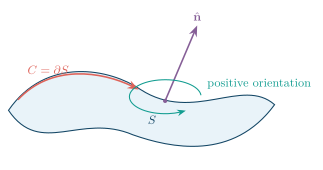
∇ ⋅ D = ρ v . \boxed{\nabla\cdot\mathbf D=\rho_v}. ∇ ⋅ D = ρ v . ∮ C F ⋅ d l = ∫ S ( ∇ × F ) ⋅ d S . \oint_C \mathbf{F}\cdot d\mathbf{l}
=\int_S (\nabla\times\mathbf{F})\cdot d\mathbf{S}. ∮ C F ⋅ d l = ∫ S ( ∇ × F ) ⋅ d S . The contour direction and surface normal follow the right-hand rule. For a fixed contour, applying the theorem to Faraday’s law gives
∮ C E ⋅ d l = − d d t ∫ S B ⋅ d S , ∫ S ( ∇ × E ) ⋅ d S = − ∫ S ∂ B ∂ t ⋅ d S . \begin{aligned}
\oint_C\mathbf E\cdot d\mathbf l
& =-\frac{d}{dt}\int_S\mathbf B\cdot d\mathbf S, \\
\int_S(\nabla\times\mathbf E)\cdot d\mathbf S
& =-\int_S\frac{\partial\mathbf B}{\partial t}\cdot d\mathbf S.
\end{aligned} ∮ C E ⋅ d l ∫ S ( ∇ × E ) ⋅ d S = − d t d ∫ S B ⋅ d S , = − ∫ S ∂ t ∂ B ⋅ d S . Since the surface is arbitrary,
∇ × E = − ∂ B ∂ t . \boxed{\nabla\times\mathbf E=-\frac{\partial\mathbf B}{\partial t}}. ∇ × E = − ∂ t ∂ B . The same conversion applied to the Ampere-Maxwell law yields
∇ × H = J + ∂ D ∂ t . \boxed{\nabla\times\mathbf H=\mathbf J+\frac{\partial\mathbf D}{\partial t}}. ∇ × H = J + ∂ t ∂ D .
Stokes theorem orientation for a boundary curve and surface normal.
Integral and differential forms.
An integral form describes the net behavior of a field over a finite curve, surface or volume, whereas the corresponding differential form describes the same law locally at a point.
Integral quantity Differential operator outward flux through a closed surface divergence circulation around a closed curve curl
The usual conversion path is
i n t e g r a l l a w ⟷ divergence theorem or Stokes’ theorem differential law . \mathrm{integral\ law}\quad
\overset{\text{divergence theorem or Stokes' theorem}}{\longleftrightarrow}
\quad \text{differential law}. integral law ⟷ divergence theorem or Stokes’ theorem differential law .