This section develops input-output models from physical laws, combines those models with block diagrams and signal-flow graphs, and then uses them to predict transient and steady-state response. Pole and zero locations are treated separately in the section.
For a linear time-invariant (LTI) system with all initial conditions set to zero, the transfer function is
G ( s ) = C ( s ) R ( s ) . \boxed{G(s)=\frac{C(s)}{R(s)}}. G ( s ) = R ( s ) C ( s ) . Here R ( s ) = L { r ( t ) } R(s)=\mathcal{L}\{r(t)\} R ( s ) = L { r ( t )} C ( s ) = L { c ( t ) } C(s)=\mathcal{L}\{c(t)\} C ( s ) = L { c ( t )} s = σ + j ω s=\sigma+j\omega s = σ + j ω
The usual transfer-function model assumes a linear, time-invariant, lumped-parameter system and zero initial conditions. For a SISO differential equation
a n d n c d t n + a n − 1 d n − 1 c d t n − 1 + ⋯ + a 1 d c d t + a 0 c = b m d m r d t m + b m − 1 d m − 1 r d t m − 1 + ⋯ + b 1 d r d t + b 0 r , \begin{aligned}
a_n\frac{\mathrm{d}^n c}{\mathrm{d}t^n}
+a_{n-1}\frac{\mathrm{d}^{n-1}c}{\mathrm{d}t^{n-1}}+\cdots+a_1\frac{\mathrm{d}c}{\mathrm{d}t}+a_0c
={}&b_m\frac{\mathrm{d}^m r}{\mathrm{d}t^m}
+b_{m-1}\frac{\mathrm{d}^{m-1}r}{\mathrm{d}t^{m-1}}+\cdots\\
&+b_1\frac{\mathrm{d}r}{\mathrm{d}t}+b_0r,
\end{aligned} a n d t n d n c + a n − 1 d t n − 1 d n − 1 c + ⋯ + a 1 d t d c + a 0 c = b m d t m d m r + b m − 1 d t m − 1 d m − 1 r + ⋯ + b 1 d t d r + b 0 r , the zero-state Laplace transform gives
Advantages Limitations Converts a differential equation into an algebraic relation in s s s Does not directly represent nonlinear or time-varying behavior. Gives the external input-output relation directly. Zero-state definition omits the response due to nonzero initial conditions. Poles and zeros expose stability and transient characteristics. Does not reveal internal state variables or physical realization. Supports block-diagram and frequency-response analysis. Different physical systems can have the same transfer function. Is independent of the particular applied input signal. The scalar ratio is primarily a SISO description; MIMO systems require a transfer matrix.
Advantages and limitations of a transfer-function model
Example — Transfer function from a differential equation
Find the transfer function when
d 2 c d t 2 + 5 d c d t + 6 c = 2 d r d t + 4 r . \frac{\mathrm{d}^2c}{\mathrm{d}t^2}+5\frac{\mathrm{d}c}{\mathrm{d}t}+6c
=2\frac{\mathrm{d}r}{\mathrm{d}t}+4r. d t 2 d 2 c + 5 d t d c + 6 c = 2 d t d r + 4 r . With zero initial conditions,
( s 2 + 5 s + 6 ) C ( s ) = ( 2 s + 4 ) R ( s ) , ∴ C ( s ) R ( s ) = 2 s + 4 s 2 + 5 s + 6 . \begin{aligned}
(s^2+5s+6)C(s)&=(2s+4)R(s),\\
\therefore\quad \frac{C(s)}{R(s)}&=
\boxed{\frac{2s+4}{s^2+5s+6}}.
\end{aligned} ( s 2 + 5 s + 6 ) C ( s ) ∴ R ( s ) C ( s ) = ( 2 s + 4 ) R ( s ) , = s 2 + 5 s + 6 2 s + 4 . A model follows from an element law plus a compatibility or balance equation. Taking the Laplace transform only after writing the physical equations makes signs, units, and initial-condition assumptions visible.
Element Time-domain relation Impedance Z ( s ) = V / I Z(s)=V/I Z ( s ) = V / I Resistor R R R v ( t ) = R i ( t ) v(t)=Ri(t) v ( t ) = R i ( t ) R R R Inductor L L L v ( t ) = L d i ( t ) / d t v(t)=L\,\mathrm{d}i(t)/\mathrm{d}t v ( t ) = L d i ( t ) / d t L s Ls L s Capacitor C C C i ( t ) = C d v ( t ) / d t i(t)=C\,\mathrm{d}v(t)/\mathrm{d}t i ( t ) = C d v ( t ) / d t 1 / ( C s ) 1/(Cs) 1/ ( C s )
Electrical element relations under zero initial conditions
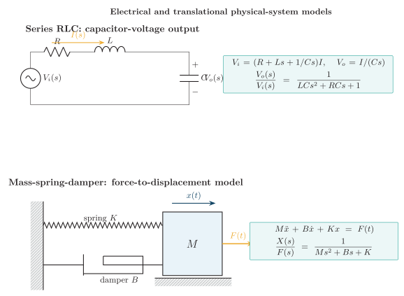
For the series RLC network of the figure, KVL and the capacitor voltage give
V i ( s ) = ( R + L s + 1 C s ) I ( s ) , V o ( s ) = I ( s ) C s . V_i(s)=\left(R+Ls+\frac{1}{Cs}\right)I(s),
\qquad V_o(s)=\frac{I(s)}{Cs}. V i ( s ) = ( R + L s + C s 1 ) I ( s ) , V o ( s ) = C s I ( s ) . Hence
V o ( s ) V i ( s ) = 1 L C s 2 + R C s + 1 . \frac{V_o(s)}{V_i(s)}=\frac{1}{LCs^2+RCs+1}. V i ( s ) V o ( s ) = L C s 2 + R C s + 1 1 . Element Force relation Coefficient for F ( s ) / X ( s ) F(s)/X(s) F ( s ) / X ( s ) Mass M M M F = M d 2 x / d t 2 F=M\,\mathrm{d}^2x/\mathrm{d}t^2 F = M d 2 x / d t 2 M s 2 Ms^2 M s 2 Viscous damper B B B F = B d x / d t F=B\,\mathrm{d}x/\mathrm{d}t F = B d x / d t B s Bs B s Linear spring K K K F = K x F=Kx F = K x K K K
Translational mechanical element relations
Newton’s law for the mass-spring-damper system is
M x ¨ ( t ) + B x ˙ ( t ) + K x ( t ) = F ( t ) . M\ddot{x}(t)+B\dot{x}(t)+Kx(t)=F(t). M x ¨ ( t ) + B x ˙ ( t ) + K x ( t ) = F ( t ) . Therefore
( M s 2 + B s + K ) X ( s ) = F ( s ) , X ( s ) F ( s ) = 1 M s 2 + B s + K . (Ms^2+Bs+K)X(s)=F(s),
\qquad
\boxed{\frac{X(s)}{F(s)}=\frac{1}{Ms^2+Bs+K}}. ( M s 2 + B s + K ) X ( s ) = F ( s ) , F ( s ) X ( s ) = M s 2 + B s + K 1 .
Electrical and mechanical models obtained from element laws and force balance.
The rotational counterparts of mass, force, and displacement are moment of inertia J J J T T T θ \theta θ
Element Torque relation Moment of inertia J J J T = J d 2 θ / d t 2 = J d ω / d t T=J\,\mathrm{d}^2\theta/\mathrm{d}t^2=J\,\mathrm{d}\omega/\mathrm{d}t T = J d 2 θ / d t 2 = J d ω / d t Viscous friction B B B T = B d θ / d t = B ω T=B\,\mathrm{d}\theta/\mathrm{d}t=B\omega T = B d θ / d t = B ω Torsional spring K K K T = K θ T=K\theta T = K θ
Rotational mechanical element relations
For a single inertia with viscous friction and a torsional spring,
J θ ¨ + B θ ˙ + K θ = T ( t ) , J\ddot{\theta}+B\dot{\theta}+K\theta=T(t), J θ ¨ + B θ ˙ + K θ = T ( t ) , so
Θ ( s ) T ( s ) = 1 J s 2 + B s + K , Ω ( s ) T ( s ) = s J s 2 + B s + K . \boxed{\frac{\Theta(s)}{T(s)}=\frac{1}{Js^2+Bs+K}},
\qquad
\frac{\Omega(s)}{T(s)}=\frac{s}{Js^2+Bs+K}. T ( s ) Θ ( s ) = J s 2 + B s + K 1 , T ( s ) Ω ( s ) = J s 2 + B s + K s . Force-voltage (impedance) analogy Force-current (mobility) analogy F ↔ V F\leftrightarrow V F ↔ V F ↔ I F\leftrightarrow I F ↔ I Velocity v ↔ i v\leftrightarrow i v ↔ i Velocity v ↔ V v\leftrightarrow V v ↔ V M ↔ L M\leftrightarrow L M ↔ L M ↔ C M\leftrightarrow C M ↔ C B ↔ R B\leftrightarrow R B ↔ R B ↔ 1 / R B\leftrightarrow 1/R B ↔ 1/ R K ↔ 1 / C K\leftrightarrow 1/C K ↔ 1/ C K ↔ 1 / L K\leftrightarrow 1/L K ↔ 1/ L
Force-voltage and force-current analogies
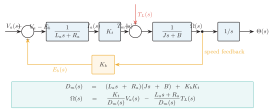
Assume constant field flux, linear operation, viscous shaft friction, and zero initial conditions. Let R a R_a R a L a L_a L a K b K_b K b K t K_t K t J J J B B B T L T_L T L
The electrical and electromechanical relations are
V a ( t ) = R a i a ( t ) + L a d i a d t + e b ( t ) , e b ( t ) = K b ω ( t ) = K b d θ d t , T m ( t ) = K t i a ( t ) . \begin{aligned}
V_a(t)&=R_ai_a(t)+L_a\frac{\mathrm{d}i_a}{\mathrm{d}t}+e_b(t),\\
e_b(t)&=K_b\omega(t)=K_b\frac{\mathrm{d}\theta}{\mathrm{d}t},\\
T_m(t)&=K_ti_a(t).
\end{aligned} V a ( t ) e b ( t ) T m ( t ) = R a i a ( t ) + L a d t d i a + e b ( t ) , = K b ω ( t ) = K b d t d θ , = K t i a ( t ) . The signed mechanical balance is
J d ω d t + B ω = T m − T L . J\frac{\mathrm{d}\omega}{\mathrm{d}t}+B\omega=T_m-T_L. J d t d ω + B ω = T m − T L . In the s s s
V a ( s ) = ( L a s + R a ) I a ( s ) + K b Ω ( s ) , ( J s + B ) Ω ( s ) = K t I a ( s ) − T L ( s ) . \begin{aligned}
V_a(s)&=(L_as+R_a)I_a(s)+K_b\Omega(s),\\
(Js+B)\Omega(s)&=K_tI_a(s)-T_L(s).
\end{aligned} V a ( s ) ( J s + B ) Ω ( s ) = ( L a s + R a ) I a ( s ) + K b Ω ( s ) , = K t I a ( s ) − T L ( s ) . Eliminating I a ( s ) I_a(s) I a ( s )
I a ( s ) = V a ( s ) − K b Ω ( s ) L a s + R a , [ ( L a s + R a ) ( J s + B ) + K b K t ] Ω ( s ) = K t V a ( s ) − ( L a s + R a ) T L ( s ) . \begin{aligned}
I_a(s)&=\frac{V_a(s)-K_b\Omega(s)}{L_as+R_a},\\
\bigl[(L_as+R_a)(Js+B)+K_bK_t\bigr]\Omega(s)
&=K_tV_a(s)-(L_as+R_a)T_L(s).
\end{aligned} I a ( s ) [ ( L a s + R a ) ( J s + B ) + K b K t ] Ω ( s ) = L a s + R a V a ( s ) − K b Ω ( s ) , = K t V a ( s ) − ( L a s + R a ) T L ( s ) . Define the motor denominator
D m ( s ) = ( L a s + R a ) ( J s + B ) + K b K t . D_m(s)=(L_as+R_a)(Js+B)+K_bK_t. D m ( s ) = ( L a s + R a ) ( J s + B ) + K b K t . Superposition then gives the complete speed relation
Consequently,
Ω ( s ) V a ( s ) ∣ T L = 0 = K t ( L a s + R a ) ( J s + B ) + K b K t , Θ ( s ) V a ( s ) ∣ T L = 0 = K t s [ ( L a s + R a ) ( J s + B ) + K b K t ] , Ω ( s ) T L ( s ) ∣ V a = 0 = − L a s + R a ( L a s + R a ) ( J s + B ) + K b K t . \begin{aligned}
\left.\frac{\Omega(s)}{V_a(s)}\right|_{T_L=0}
&=\boxed{\frac{K_t}{(L_as+R_a)(Js+B)+K_bK_t}},\\
\left.\frac{\Theta(s)}{V_a(s)}\right|_{T_L=0}
&=\boxed{\frac{K_t}{s\bigl[(L_as+R_a)(Js+B)+K_bK_t\bigr]}},\\
\left.\frac{\Omega(s)}{T_L(s)}\right|_{V_a=0}
&=\boxed{-\frac{L_as+R_a}{(L_as+R_a)(Js+B)+K_bK_t}}.
\end{aligned} V a ( s ) Ω ( s ) T L = 0 V a ( s ) Θ ( s ) T L = 0 T L ( s ) Ω ( s ) V a = 0 = ( L a s + R a ) ( J s + B ) + K b K t K t , = s [ ( L a s + R a ) ( J s + B ) + K b K t ] K t , = − ( L a s + R a ) ( J s + B ) + K b K t L a s + R a . The minus sign in the last expression is a consequence of the chosen opposing-load convention. If L a L_a L a
Ω ( s ) V a ( s ) ≈ K t R a J s + R a B + K b K t . \frac{\Omega(s)}{V_a(s)}\approx
\boxed{\frac{K_t}{R_aJs+R_aB+K_bK_t}}. V a ( s ) Ω ( s ) ≈ R a J s + R a B + K b K t K t .
Exam Focus — Motor signs and SI units
K t K_t K t N m / A \mathrm{N\,m/A} N m/A K b K_b K b V s / r a d \mathrm{V\,s/rad} V s/rad T m − T L T_m-T_L T m − T L
Armature-controlled DC motor model with back-emf feedback, load-torque disturbance, speed output, and position integrator.
A block diagram represents functional input-output relations and the direction of signal flow. Reduction preserves the relation between the selected external input and output.
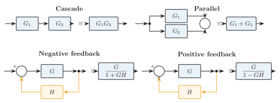
Connection Equivalent transfer Condition Cascade G 1 G 2 G_1G_2 G 1 G 2 The same signal passes through both blocks Parallel paths G 1 + G 2 G_1+G_2 G 1 + G 2 Branch outputs enter an additive summing point Negative feedback G / ( 1 + G H ) G/(1+GH) G / ( 1 + G H ) Feedback enters the comparator with a minus sign Positive feedback G / ( 1 − G H ) G/(1-GH) G / ( 1 − G H ) Feedback enters the comparator with a plus sign
Basic block-diagram equivalents
Basic cascade, parallel, and feedback reduction rules.
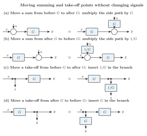
Moving a summing or take-off point across a block requires compensation:
moving a sum from before G G G G G G G G G
moving a sum from after G G G G G G 1 / G 1/G 1/ G
moving a take-off from before G G G G G G 1 / G 1/G 1/ G
moving a take-off from after G G G G G G G G G
In every case, verify the signal carried by the moved branch rather than memorizing the picture alone.
Compensating gains when a summing or take-off point is moved across a block.
Combine obvious cascade blocks.
Combine parallel blocks that share the same input and summing point.
Reduce the innermost feedback loop first.
Move summing or take-off points only when a loop cannot otherwise be isolated.
Repeat until one equivalent block remains, then check limiting cases and signs.
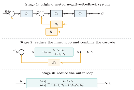
In the figure, G 2 G_2 G 2 H 1 H_1 H 1 H 2 H_2 H 2
G i n = G 2 1 + G 2 H 1 . G_{\mathrm{in}}=\frac{G_2}{1+G_2H_1}. G in = 1 + G 2 H 1 G 2 . The resulting cascade is
G e q = G 1 G i n G 3 = G 1 G 2 G 3 1 + G 2 H 1 . G_{\mathrm{eq}}=G_1G_{\mathrm{in}}G_3
=\frac{G_1G_2G_3}{1+G_2H_1}. G eq = G 1 G in G 3 = 1 + G 2 H 1 G 1 G 2 G 3 . Finally reduce the outer loop:
C ( s ) R ( s ) = G e q 1 + G e q H 2 = G 1 G 2 G 3 1 + G 2 H 1 + G 1 G 2 G 3 H 2 . \begin{aligned}
\frac{C(s)}{R(s)}
&=\frac{G_{\mathrm{eq}}}{1+G_{\mathrm{eq}}H_2}\\
&=\boxed{\frac{G_1G_2G_3}
{1+G_2H_1+G_1G_2G_3H_2}}.
\end{aligned} R ( s ) C ( s ) = 1 + G eq H 2 G eq = 1 + G 2 H 1 + G 1 G 2 G 3 H 2 G 1 G 2 G 3 .
Worked reduction of nested negative-feedback loops from the inner loop outward.
A signal-flow graph (SFG) represents a set of linear algebraic relations by signal nodes and directed branches whose transmittances multiply the signal at the branch tail.
Term Meaning Node A system variable or signal Branch Directed connection from one node to another Branch gain Transmittance multiplying the signal along a branch Source (input) node Node having outgoing branches but no incoming branch Sink (output) node Node having incoming branches but no outgoing branch Forward path Source-to-sink path that does not pass through any node more than once Loop Closed path that begins and ends at one node without repeating any other node Non-touching loops Loops that share no node
Signal-flow graph terminology
Law — Mason’s gain formula
If P k P_k P k k k k
T = C ( s ) R ( s ) = ∑ k = 1 N P k Δ k Δ . \boxed{T=\frac{C(s)}{R(s)}=
\frac{\displaystyle\sum_{k=1}^{N}P_k\Delta_k}{\Delta}}. T = R ( s ) C ( s ) = Δ k = 1 ∑ N P k Δ k . The graph determinant is
Δ = 1 − ∑ i L i + ∑ i < j L i L j − ∑ i < j < ℓ L i L j L ℓ + ⋯ , \Delta=1-\sum_i L_i
+\sum_{i<j}L_iL_j
-\sum_{i<j<\ell}L_iL_jL_\ell+\cdots, Δ = 1 − i ∑ L i + i < j ∑ L i L j − i < j < ℓ ∑ L i L j L ℓ + ⋯ , where a product is included only when all loops in that product are mutually non-touching. The cofactor Δ k \Delta_k Δ k P k P_k P k
List every forward path and calculate each path gain P k P_k P k
List every individual loop and its signed loop gain L i L_i L i
Identify all pairs, triples, and higher groups of non-touching loops.
Form the graph determinant Δ \Delta Δ
Form each path cofactor Δ k \Delta_k Δ k P k P_k P k
Substitute in Mason’s formula and simplify.
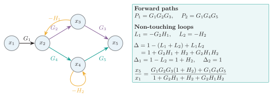
For the figure, the two forward paths are
P 1 = G 1 G 2 G 3 , P 2 = G 1 G 4 G 5 . P_1=G_1G_2G_3,\qquad P_2=G_1G_4G_5. P 1 = G 1 G 2 G 3 , P 2 = G 1 G 4 G 5 . The loop gains are L 1 = − G 2 H 1 L_1=-G_2H_1 L 1 = − G 2 H 1 { x 2 , x 3 } \{x_2,x_3\} { x 2 , x 3 } L 2 = − H 2 L_2=-H_2 L 2 = − H 2 x 4 x_4 x 4
Δ = 1 − ( L 1 + L 2 ) + L 1 L 2 = 1 + G 2 H 1 + H 2 + G 2 H 1 H 2 . \begin{aligned}
\Delta&=1-(L_1+L_2)+L_1L_2\\
&=1+G_2H_1+H_2+G_2H_1H_2.
\end{aligned} Δ = 1 − ( L 1 + L 2 ) + L 1 L 2 = 1 + G 2 H 1 + H 2 + G 2 H 1 H 2 . Path P 1 P_1 P 1 L 1 L_1 L 1 L 2 L_2 L 2 P 2 P_2 P 2
Δ 1 = 1 − L 2 = 1 + H 2 , Δ 2 = 1 , \Delta_1=1-L_2=1+H_2,\qquad \Delta_2=1, Δ 1 = 1 − L 2 = 1 + H 2 , Δ 2 = 1 , and
x 5 x 1 = G 1 G 2 G 3 ( 1 + H 2 ) + G 1 G 4 G 5 1 + G 2 H 1 + H 2 + G 2 H 1 H 2 . \boxed{\frac{x_5}{x_1}=
\frac{G_1G_2G_3(1+H_2)+G_1G_4G_5}
{1+G_2H_1+H_2+G_2H_1H_2}}. x 1 x 5 = 1 + G 2 H 1 + H 2 + G 2 H 1 H 2 G 1 G 2 G 3 ( 1 + H 2 ) + G 1 G 4 G 5 .
Signal-flow graph with two forward paths and two non-touching loops, evaluated using Mason’s formula.
Standard inputs make the performance of different systems directly comparable.
Input Time function Laplace transform Main use Impulse δ ( t ) \delta(t) δ ( t ) 1 1 1 Reveals the impulse response directly Step u ( t ) u(t) u ( t ) 1 / s 1/s 1/ s Tests set-point regulation Ramp t u ( t ) t\,u(t) t u ( t ) 1 / s 2 1/s^2 1/ s 2 Tests constant-velocity tracking Parabolic t 2 u ( t ) / 2 t^2u(t)/2 t 2 u ( t ) /2 1 / s 3 1/s^3 1/ s 3 Tests constant-acceleration tracking Sinusoid sin ( ω t ) u ( t ) \sin(\omega t)u(t) sin ( ω t ) u ( t ) ω / ( s 2 + ω 2 ) \omega/(s^2+\omega^2) ω / ( s 2 + ω 2 ) Tests frequency response
Unit test signals and their one-sided Laplace transforms
The output is commonly separated as
c ( t ) = c t r ( t ) + c s s ( t ) , c(t)=c_{\mathrm{tr}}(t)+c_{\mathrm{ss}}(t), c ( t ) = c tr ( t ) + c ss ( t ) , where the transient component contains decaying natural modes and the steady-state component remains after those modes vanish.
The normalized stable first-order prototype is
For a unit step R ( s ) = 1 / s R(s)=1/s R ( s ) = 1/ s
C ( s ) = 1 s ( T s + 1 ) = 1 s − 1 s + 1 / T , c ( t ) = 1 − e − t / T , t ≥ 0. \begin{aligned}
C(s)&=\frac{1}{s(Ts+1)}
=\frac{1}{s}-\frac{1}{s+1/T},\\
c(t)&=\boxed{1-e^{-t/T}},\qquad t\geq0.
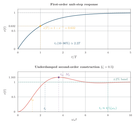
\end{aligned} C ( s ) c ( t ) = s ( T s + 1 ) 1 = s 1 − s + 1/ T 1 , = 1 − e − t / T , t ≥ 0. At t = T t=T t = T e − 1 e^{-1} e − 1 63.2 % 63.2\% 63.2%
t t t T T T 2 T 2T 2 T 3 T 3T 3 T 4 T 4T 4 T 5 T 5T 5 T c ( t ) c(t) c ( t ) 0.632 0.632 0.632 0.865 0.865 0.865 0.950 0.950 0.950 0.982 0.982 0.982 0.993 0.993 0.993
First-order step-response landmarks
Solving c ( t ) = q c(t)=q c ( t ) = q t q = − T ln ( 1 − q ) t_q=-T\ln(1-q) t q = − T ln ( 1 − q )
t d = T ln 2 = 0.693 T (time to 50 % ) , t r = t 90 − t 10 = T ln 9 = 2.197 T ≈ 2.2 T , t s ( 2 % ) = − T ln ( 0.02 ) = 3.912 T ≈ 4 T , t s ( 5 % ) = − T ln ( 0.05 ) = 2.996 T ≈ 3 T . \begin{aligned}
t_d&=T\ln2=0.693T &&\text{(time to $50\%$)},\\
t_r&=t_{90}-t_{10}=T\ln9=2.197T\approx2.2T,\\
t_s(2\%)&=-T\ln(0.02)=3.912T\approx4T,\\
t_s(5\%)&=-T\ln(0.05)=2.996T\approx3T.
\end{aligned} t d t r t s ( 2% ) t s ( 5% ) = T ln 2 = 0.693 T = t 90 − t 10 = T ln 9 = 2.197 T ≈ 2.2 T , = − T ln ( 0.02 ) = 3.912 T ≈ 4 T , = − T ln ( 0.05 ) = 2.996 T ≈ 3 T . (time to 50%) , The first-order prototype is monotonic, so it has no finite peak time or overshoot.
The unity-DC-gain second-order closed-loop prototype is
The characteristic roots are
s 1 , 2 = − ζ ω n ± ω n ζ 2 − 1 . s_{1,2}=-\zeta\omega_n
\pm\omega_n\sqrt{\zeta^2-1}. s 1 , 2 = − ζ ω n ± ω n ζ 2 − 1 . For 0 < ζ < 1 0<\zeta<1 0 < ζ < 1
s 1 , 2 = − ζ ω n ± j ω d , ω d = ω n 1 − ζ 2 . s_{1,2}=-\zeta\omega_n\pm j\omega_d,
\qquad \boxed{\omega_d=\omega_n\sqrt{1-\zeta^2}}. s 1 , 2 = − ζ ω n ± j ω d , ω d = ω n 1 − ζ 2 . Their geometry is shown in the figure.
With R ( s ) = 1 / s R(s)=1/s R ( s ) = 1/ s
C ( s ) = ω n 2 s ( s 2 + 2 ζ ω n s + ω n 2 ) = 1 s − s + 2 ζ ω n s 2 + 2 ζ ω n s + ω n 2 . \begin{aligned}
C(s)&=\frac{\omega_n^2}
{s(s^2+2\zeta\omega_ns+\omega_n^2)}\\
&=\frac{1}{s}-
\frac{s+2\zeta\omega_n}{s^2+2\zeta\omega_ns+\omega_n^2}.
\end{aligned} C ( s ) = s ( s 2 + 2 ζ ω n s + ω n 2 ) ω n 2 = s 1 − s 2 + 2 ζ ω n s + ω n 2 s + 2 ζ ω n . Completing the square in the quadratic denominator and inverting term by term gives
c ( t ) = 1 − e − ζ ω n t [ cos ( ω d t ) + ζ 1 − ζ 2 sin ( ω d t ) ] = 1 − e − ζ ω n t 1 − ζ 2 sin ( ω d t + ϕ ) , \begin{aligned}
c(t)&=1-e^{-\zeta\omega_nt}
\left[\cos(\omega_dt)+
\frac{\zeta}{\sqrt{1-\zeta^2}}\sin(\omega_dt)\right]\\
&=\boxed{1-
\frac{e^{-\zeta\omega_nt}}{\sqrt{1-\zeta^2}}
\sin(\omega_dt+\phi)},
\end{aligned} c ( t ) = 1 − e − ζ ω n t [ cos ( ω d t ) + 1 − ζ 2 ζ sin ( ω d t ) ] = 1 − 1 − ζ 2 e − ζ ω n t sin ( ω d t + ϕ ) , where
ϕ = cos − 1 ζ = tan − 1 ( 1 − ζ 2 ζ ) , 0 < ζ < 1. \phi=\cos^{-1}\zeta
=\tan^{-1}\!\left(\frac{\sqrt{1-\zeta^2}}{\zeta}\right),
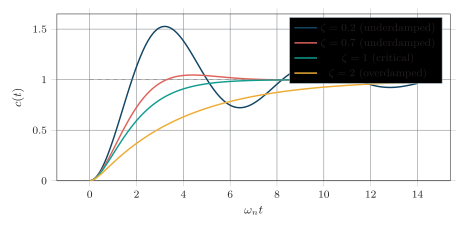
\qquad 0<\zeta<1. ϕ = cos − 1 ζ = tan − 1 ( ζ 1 − ζ 2 ) , 0 < ζ < 1. Damping ratio Poles Unit-step behavior ζ < 0 \zeta<0 ζ < 0 At least one pole in RHP Growing, unstable response ζ = 0 \zeta=0 ζ = 0 ± j ω n \pm j\omega_n ± j ω n Undamped oscillation, c ( t ) = 1 − cos ω n t c(t)=1-\cos\omega_nt c ( t ) = 1 − cos ω n t 0 < ζ < 1 0<\zeta<1 0 < ζ < 1 Complex-conjugate LHP pair Decaying oscillation with overshoot ζ = 1 \zeta=1 ζ = 1 Repeated pole at − ω n -\omega_n − ω n Critical response 1 − ( 1 + ω n t ) e − ω n t 1-(1+\omega_nt)e^{-\omega_nt} 1 − ( 1 + ω n t ) e − ω n t ζ > 1 \zeta>1 ζ > 1 Two real LHP poles Slow, nonoscillatory overdamped response
Second-order damping cases
For ζ > 1 \zeta>1 ζ > 1
p 1 , 2 = − ω n ( ζ ∓ ζ 2 − 1 ) . p_{1,2}=-\omega_n\left(\zeta\mp\sqrt{\zeta^2-1}\right). p 1 , 2 = − ω n ( ζ ∓ ζ 2 − 1 ) . Then the overdamped unit-step response can be written
c ( t ) = 1 + p 2 e p 1 t − p 1 e p 2 t p 1 − p 2 . c(t)=1+\frac{p_2e^{p_1t}-p_1e^{p_2t}}{p_1-p_2}. c ( t ) = 1 + p 1 − p 2 p 2 e p 1 t − p 1 e p 2 t .
Unit-step responses of the normalized second-order prototype for representative damping ratios.
Let c ( ∞ ) = 1 c(\infty)=1 c ( ∞ ) = 1 0 < ζ < 1 0<\zeta<1 0 < ζ < 1
Specification Symbol Definition or result Delay time t d t_d t d First time the response reaches 50 % 50\% 50% Rise time t r t_r t r First 0 0 0 100 % 100\% 100% ( π − ϕ ) / ω d (\pi-\phi)/\omega_d ( π − ϕ ) / ω d Peak time t p t_p t p First maximum: π / ω d \pi/\omega_d π / ω d Maximum overshoot M p M_p M p ( c max − c ∞ ) / c ∞ = e − π ζ / 1 − ζ 2 (c_{\max}-c_\infty)/c_\infty=e^{-\pi\zeta/\sqrt{1-\zeta^2}} ( c m a x − c ∞ ) / c ∞ = e − π ζ / 1 − ζ 2 Percent overshoot % O S \%OS % O S 100 e − π ζ / 1 − ζ 2 100e^{-\pi\zeta/\sqrt{1-\zeta^2}} 100 e − π ζ / 1 − ζ 2 Settling time t s t_s t s Time after which the response remains inside a specified tolerance band
Underdamped second-order time-domain specifications
The oscillatory error is bounded by
∣ 1 − c ( t ) ∣ ≤ e − ζ ω n t 1 − ζ 2 . |1-c(t)|\leq
\frac{e^{-\zeta\omega_nt}}{\sqrt{1-\zeta^2}}. ∣1 − c ( t ) ∣ ≤ 1 − ζ 2 e − ζ ω n t . Thus an envelope-based tolerance estimate is
t s ( ε ) = − ln ( ε 1 − ζ 2 ) ζ ω n . t_s(\varepsilon)=
\frac{-\ln\!\left(\varepsilon\sqrt{1-\zeta^2}\right)}
{\zeta\omega_n}. t s ( ε ) = ζ ω n − ln ( ε 1 − ζ 2 ) . The frequently used textbook approximations are
They neglect the factor 1 / 1 − ζ 2 1/\sqrt{1-\zeta^2} 1/ 1 − ζ 2 ζ = 0 \zeta=0 ζ = 0 ζ = 1 \zeta=1 ζ = 1
Increasing ζ \zeta ζ ζ \zeta ζ ω n \omega_n ω n ζ ω n \zeta\omega_n ζ ω n
First-order time constant and second-order delay, rise, peak, overshoot, and settling constructions.
Example — Second-order response specifications
A standard second-order system has ζ = 0.5 \zeta=0.5 ζ = 0.5 ω n = 10 r a d / s \omega_n=10\,\mathrm{rad/s} ω n = 10 rad/s ω d \omega_d ω d t p t_p t p 2 % 2\% 2%
ω d = 10 1 − 0.5 2 = 8.66 r a d / s , t p = π 8.66 = 0.363 s , % O S = 100 e − π ( 0.5 ) / 1 − 0.5 2 = 16.3 % , t s ( 2 % ) ≈ 4 0.5 ( 10 ) = 0.80 s . \begin{aligned}
\omega_d&=10\sqrt{1-0.5^2}=8.66\,\mathrm{rad/s},\\
t_p&=\frac{\pi}{8.66}=0.363\,\mathrm{s},\\
\%OS&=100e^{-\pi(0.5)/\sqrt{1-0.5^2}}=16.3\%,\\
t_s(2\%)&\approx\frac{4}{0.5(10)}=0.80\,\mathrm{s}.
\end{aligned} ω d t p % O S t s ( 2% ) = 10 1 − 0. 5 2 = 8.66 rad/s , = 8.66 π = 0.363 s , = 100 e − π ( 0.5 ) / 1 − 0. 5 2 = 16.3% , ≈ 0.5 ( 10 ) 4 = 0.80 s . Using the full envelope expression gives about 0.811 s 0.811\,\mathrm{s} 0.811 s 0.80 s 0.80\,\mathrm{s} 0.80 s
If the limit exists, the steady-state error is
e s s = lim t → ∞ e ( t ) . \boxed{e_{ss}=\lim_{t\to\infty}e(t)}. e ss = t → ∞ lim e ( t ) . For a negative-feedback system with loop transfer L ( s ) = G ( s ) H ( s ) L(s)=G(s)H(s) L ( s ) = G ( s ) H ( s )
E ( s ) = R ( s ) 1 + L ( s ) . E(s)=\frac{R(s)}{1+L(s)}. E ( s ) = 1 + L ( s ) R ( s ) . For unity feedback, H ( s ) = 1 H(s)=1 H ( s ) = 1 L ( s ) = G ( s ) L(s)=G(s) L ( s ) = G ( s )
The final-value theorem gives
Key Formula — Final-value evaluation
e s s = lim s → 0 s E ( s ) = lim s → 0 s R ( s ) 1 + L ( s ) . e_{ss}=\lim_{s\to0}sE(s)
=\lim_{s\to0}\frac{sR(s)}{1+L(s)}. e ss = s → 0 lim s E ( s ) = s → 0 lim 1 + L ( s ) s R ( s ) . [!NOTE]
Law — Final-value theorem condition
The limit above is valid only when every pole of s E ( s ) sE(s) s E ( s )
For the standard unit polynomial inputs, define the static error constants
K p = lim s → 0 L ( s ) , K v = lim s → 0 s L ( s ) , K a = lim s → 0 s 2 L ( s ) . \boxed{K_p=\lim_{s\to0}L(s)},\qquad
\boxed{K_v=\lim_{s\to0}sL(s)},\qquad
\boxed{K_a=\lim_{s\to0}s^2L(s)}. K p = s → 0 lim L ( s ) , K v = s → 0 lim s L ( s ) , K a = s → 0 lim s 2 L ( s ) . Input R ( s ) R(s) R ( s ) Relevant constant e s s e_{ss} e ss Unit step 1 / s 1/s 1/ s K p = lim s → 0 L ( s ) K_p=\lim_{s\to0}L(s) K p = lim s → 0 L ( s ) 1 / ( 1 + K p ) 1/(1+K_p) 1/ ( 1 + K p ) Unit ramp 1 / s 2 1/s^2 1/ s 2 K v = lim s → 0 s L ( s ) K_v=\lim_{s\to0}sL(s) K v = lim s → 0 s L ( s ) 1 / K v 1/K_v 1/ K v Unit parabolic 1 / s 3 1/s^3 1/ s 3 K a = lim s → 0 s 2 L ( s ) K_a=\lim_{s\to0}s^2L(s) K a = lim s → 0 s 2 L ( s ) 1 / K a 1/K_a 1/ K a
Static error constants for a stable negative-feedback loop
Here 1 / 0 1/0 1/0 1 / ∞ = 0 1/\infty=0 1/∞ = 0
The system type is the number of uncancelled poles at the origin in the loop transfer L ( s ) = G ( s ) H ( s ) L(s)=G(s)H(s) L ( s ) = G ( s ) H ( s )
Type Origin poles Step Ramp Parabolic 0 1 / ( 1 + K p ) 1/(1+K_p) 1/ ( 1 + K p ) ∞ \infty ∞ ∞ \infty ∞ 1 1 0 0 0 1 / K v 1/K_v 1/ K v ∞ \infty ∞ 2 2 0 0 0 0 0 0 1 / K a 1/K_a 1/ K a
System type and unit-input steady-state error
Increasing type improves low-frequency tracking accuracy, but each added integrator contributes phase lag and can reduce relative stability. It is therefore not valid to improve error performance without rechecking the closed-loop characteristic equation.
Example — Steady-state error of a Type 1 system
For negative unity feedback with
G ( s ) = 10 s ( s + 2 ) , G(s)=\frac{10}{s(s+2)}, G ( s ) = s ( s + 2 ) 10 , find the error constants and the unit-step and unit-ramp errors. The closed-loop characteristic polynomial is s ( s + 2 ) + 10 = s 2 + 2 s + 10 s(s+2)+10=s^2+2s+10 s ( s + 2 ) + 10 = s 2 + 2 s + 10 − 1 -1 − 1
K p = lim s → 0 10 s ( s + 2 ) = ∞ , e s s , s t e p = 1 1 + K p = 0 , K v = lim s → 0 10 s + 2 = 5 , e s s , r a m p = 1 K v = 0.2 , K a = lim s → 0 10 s s + 2 = 0 , e s s , p a r a b o l i c = ∞ . \begin{aligned}
K_p&=\lim_{s\to0}\frac{10}{s(s+2)}=\infty,
&e_{ss,\mathrm{step}}&=\frac{1}{1+K_p}=0,\\
K_v&=\lim_{s\to0}\frac{10}{s+2}=5,
&e_{ss,\mathrm{ramp}}&=\frac{1}{K_v}=0.2,\\
K_a&=\lim_{s\to0}\frac{10s}{s+2}=0,
&e_{ss,\mathrm{parabolic}}&=\infty.
\end{aligned} K p K v K a = s → 0 lim s ( s + 2 ) 10 = ∞ , = s → 0 lim s + 2 10 = 5 , = s → 0 lim s + 2 10 s = 0 , e ss , step e ss , ramp e ss , parabolic = 1 + K p 1 = 0 , = K v 1 = 0.2 , = ∞. The last result is included to complete the error-constant classification, although only step and ramp errors were requested.
Topic Key result Transfer function G ( s ) = C ( s ) / R ( s ) G(s)=C(s)/R(s) G ( s ) = C ( s ) / R ( s ) Pole and zero Denominator and numerator roots; see the section Stable pole region All uncancelled poles strictly in the LHP for BIBO stability Mass-spring-damper X / F = 1 / ( M s 2 + B s + K ) X/F=1/(Ms^2+Bs+K) X / F = 1/ ( M s 2 + B s + K ) DC motor speed Ω / V a = K t / [ ( L a s + R a ) ( J s + B ) + K b K t ] \Omega/V_a=K_t/[(L_as+R_a)(Js+B)+K_bK_t] Ω/ V a = K t / [( L a s + R a ) ( J s + B ) + K b K t ] DC motor disturbance Ω / T L = − ( L a s + R a ) / [ ( L a s + R a ) ( J s + B ) + K b K t ] \Omega/T_L=-(L_as+R_a)/[(L_as+R_a)(Js+B)+K_bK_t] Ω/ T L = − ( L a s + R a ) / [( L a s + R a ) ( J s + B ) + K b K t ] Cascade and parallel G 1 G 2 G_1G_2 G 1 G 2 G 1 + G 2 G_1+G_2 G 1 + G 2 Negative feedback G / ( 1 + G H ) G/(1+GH) G / ( 1 + G H ) Mason formula T = ∑ k P k Δ k / Δ T=\sum_kP_k\Delta_k/\Delta T = ∑ k P k Δ k /Δ First-order step c ( t ) = 1 − e − t / T c(t)=1-e^{-t/T} c ( t ) = 1 − e − t / T First-order timing t r ( 10 t_r(10 t r ( 10 90 % ) ≈ 2.2 T 90\%)\approx2.2T 90% ) ≈ 2.2 T t s ( 2 % ) ≈ 4 T t_s(2\%)\approx4T t s ( 2% ) ≈ 4 T Second-order prototype ω n 2 / ( s 2 + 2 ζ ω n s + ω n 2 ) \omega_n^2/(s^2+2\zeta\omega_ns+\omega_n^2) ω n 2 / ( s 2 + 2 ζ ω n s + ω n 2 ) Damped frequency ω d = ω n 1 − ζ 2 \omega_d=\omega_n\sqrt{1-\zeta^2} ω d = ω n 1 − ζ 2 Peak time t p = π / ω d t_p=\pi/\omega_d t p = π / ω d Percent overshoot 100 e − π ζ / 1 − ζ 2 100e^{-\pi\zeta/\sqrt{1-\zeta^2}} 100 e − π ζ / 1 − ζ 2 Approximate 2 % 2\% 2% t s ≈ 4 / ( ζ ω n ) t_s\approx4/(\zeta\omega_n) t s ≈ 4/ ( ζ ω n ) Error constants K p = lim L K_p=\lim L K p = lim L K v = lim s L K_v=\lim sL K v = lim s L K a = lim s 2 L K_a=\lim s^2L K a = lim s 2 L s → 0 s\to0 s → 0 System type Number of uncancelled pure integrators in L ( s ) = G ( s ) H ( s ) L(s)=G(s)H(s) L ( s ) = G ( s ) H ( s )
Transfer-function and response revision table
Key Point — Quick review
A transfer function is a zero-state input-output description, not a complete internal-state model.
Poles generate natural modes and decide BIBO stability; zeros reshape the forced response and may create inverse response.
Dominant poles are the slow, appreciably excited poles nearest the imaginary axis, not merely the nearest symbols on a plot.
Standard second-order formulas apply to the normalized prototype and use clearly stated rise- and settling-band conventions.
System type predicts polynomial tracking error only after closed-loop stability and the final-value theorem conditions have been verified.
The four worked examples are distributed by topic: transfer-function formation, pole-zero interpretation in the section, second-order timing, and steady-state error.