Hilbert Transform

The Hilbert transform constructs a quadrature companion to a signal. Its principal uses are analytic-signal formation, envelope and phase analysis, and single-sideband (SSB) generation. The transform is a singular convolution in time and a sign-dependent phase rotation in frequency. This section uses the Fourier convention already established in Section 4, $X(\omega)=\int_{-\infty}^{\infty}x(t)e^{-\mathrm{j}\omega t}\mathrm{d}t$ , without repeating the broader Fourier theory.

The Hilbert transform of $x(t)$ is
$\hat{x}(t)=\mathcal H\{x(t)\} =\frac{1}{\pi}\operatorname{PV} \int_{-\infty}^{\infty}\frac{x(\tau)}{t-\tau}\,\mathrm{d}\tau.$
Here $\operatorname{PV}$ denotes the Cauchy principal value; the ordinary integral is generally undefined because its kernel is singular at $\tau=t$ .

For a sufficiently well-behaved signal, the principal value means the symmetric limiting process

\operatorname{PV}\int_{-\infty}^{\infty} \frac{x(\tau)}{t-\tau}\,\mathrm{d}\tau =\lim_{R\to\infty}\lim_{\epsilon\downarrow0} \left[ \int_{t-R}^{t-\epsilon}\frac{x(\tau)}{t-\tau}\,\mathrm{d}\tau +\int_{t+\epsilon}^{t+R}\frac{x(\tau)}{t-\tau}\,\mathrm{d}\tau \right].

The equal exclusion on the two sides allows the singular contributions to cancel. Replacing the principal value by an ordinary improper integral is a fundamental error.

The same definition can be written as the convolution

The kernel is understood as a distribution. Pointwise existence follows under standard smoothness and decay conditions. More generally, $\mathcal H$ is bounded on $L^p(\mathbb R)$ for $1<p<\infty$ ; in particular, every finite-energy signal in $L^2$ has a Hilbert transform in the mean-square sense even when the pointwise integral requires care.

Frequency-Domain Interpretation

If $x(t)\leftrightarrow X(\omega)$ and $\hat{x}(t)\leftrightarrow \hat{X}(\omega)$ , then

The adopted DC convention is $\operatorname{sgn}(0)=0$ , so

H_{\mathrm H}(\omega)= \begin{cases} e^{-\mathrm{j}\pi/2}=-\mathrm{j}, & \omega>0,\\ 0, & \omega=0,\\ e^{+\mathrm{j}\pi/2}=+\mathrm{j}, & \omega<0. \end{cases}

At DC the response has zero magnitude and no phase, so a pure constant is mapped to zero. For an ordinary $L^2$ spectrum, changing the response at the single point $\omega=0$ does not alter the time signal. The convention does matter for a constant or for the discrete DC line of a periodic signal.

Transform Pairs and the Double Transform

For a nonzero-frequency complex exponential,

Consequently, for $\omega_0>0$ and arbitrary phase $\phi$ ,

These signs should be derived rather than guessed: split a sinusoid into its positive- and negative-frequency exponentials and apply the two multipliers separately.

Applying the transform twice gives $[-\mathrm{j}\operatorname{sgn}(\omega)]^2=-1$ away from DC. If $x(t)=x_{\mathrm{DC}}+x_{\mathrm{AC}}(t)$ , then

For a periodic signal, $x_{\mathrm{DC}}$ is its mean. For an $L^2$ signal there is no persistent constant component, so $\mathcal H^2\{x\}=-x$ in the mean-square sense and $\mathcal H^{-1}=-\mathcal H$ .

Energy, Orthogonality, and Operator Properties

For any finite-energy signal, the unit magnitude of the multiplier almost everywhere gives

E_{\hat{x}} =\frac{1}{2\pi}\int_{-\infty}^{\infty} |\hat{X}(\omega)|^2\,\mathrm{d}\omega =\frac{1}{2\pi}\int_{-\infty}^{\infty} |X(\omega)|^2\,\mathrm{d}\omega =E_x.

If $x(t)$ is also real, $|X(\omega)|^2$ is even, and

\int_{-\infty}^{\infty}x(t)\hat{x}(t)\,\mathrm{d}t =-\frac{\mathrm{j}}{2\pi}\int_{-\infty}^{\infty} \operatorname{sgn}(\omega)|X(\omega)|^2\,\mathrm{d}\omega=0.

Thus a real finite-energy signal and its Hilbert transform are orthogonal in the global inner-product sense.

The following identities hold whenever the displayed operations and transforms exist; $a$ in the scaling row is real and nonzero.

Property	Result
Linearity	$\mathcal H\{a_1x_1+a_2x_2\}=a_1\hat{x}_1+a_2\hat{x}_2$
Time shift	$\mathcal H\{x(t-t_0)\}=\hat{x}(t-t_0)$
Time scaling	$\mathcal H\{x(at)\}=\operatorname{sgn}(a)\hat{x}(at)$
Differentiation	$\mathcal H\{\frac{\mathrm{d}x}{\mathrm{d}t}\}=\frac{\mathrm{d}}{\mathrm{d}t}\mathcal H\{x\}$
Convolution	$\mathcal H\{xy\}=\hat{x}y=x*\hat{y}$
Parity for real signals	Even $x$ gives odd $\hat{x}$ ; odd $x$ gives even $\hat{x}$
Inverse on the AC subspace	$\mathcal H^{-1}=-\mathcal H$

Analytic Signal

For a real signal $x(t)$ , its analytic signal is
$x_a(t)=x(t)+\mathrm{j}\hat{x}(t).$
Its real part is the original signal and its imaginary part is the Hilbert transform.

Because $\hat{X}(\omega)=-\mathrm{j}\operatorname{sgn}(\omega)X(\omega)$ ,

Thus negative frequencies are suppressed, positive frequencies are doubled, and DC is retained once. These factors ensure

x(t)=\Re\{x_a(t)\} =\frac{x_a(t)+x_a^*(t)}{2}.

The shorthand $X_a(\omega)=2u(\omega)X(\omega)$ is correct only with the symmetric convention $u(0)=1/2$ ; otherwise it doubles or deletes DC incorrectly.

For a real finite-energy signal, the positive and negative frequency halves contain equal energy. Doubling one half gives

E_{x_a}=2E_x.

For a real periodic signal with mean $\bar{x}$ , the corresponding power result is $P_{x_a}=2P_x-|\bar{x}|^2$ , because its DC line is not doubled.

Envelope, Instantaneous Phase, and Frequency

Where $x_a(t)\neq0$ , write the analytic signal in polar form:

Key Formula — Instantaneous signal quantities

\begin{aligned} x_a(t)&=A(t)e^{\mathrm{j}\phi(t)},\\ A(t)&=|x_a(t)| =\sqrt{x^2(t)+\hat{x}^{\,2}(t)},\\ \phi(t)&=\arg x_a(t) =\operatorname{atan2}\!\bigl(\hat{x}(t),x(t)\bigr),\\ \omega_i(t)&=\frac{\mathrm{d}\phi(t)}{\mathrm{d}t} =\operatorname{Im}\!\left\{\frac{\dot{x}_a(t)}{x_a(t)}\right\}\\ &=\frac{x(t)\dot{\hat{x}}(t)-\hat{x}(t)\dot{x}(t)} {x^2(t)+\hat{x}^{\,2}(t)},\\ f_i(t)&=\frac{\omega_i(t)}{2\pi}. \end{aligned}

The phase must be unwrapped before differentiation. These definitions also require $A(t)>0$ and sufficient differentiability. More importantly, they have a clear physical interpretation mainly for a monocomponent or suitably narrowband AM–FM signal. For a multicomponent waveform, $A(t)$ can show beating and $\omega_i(t)$ can become erratic or even negative; computability alone does not guarantee a useful physical interpretation.

Law — Bedrosian theorem and the envelope condition

Let $f(t)$ be lowpass with $F(\omega)=0$ for $|\omega|>\Omega_L$ , and let $g(t)$ be highpass with $G(\omega)=0$ for $|\omega|<\Omega_H$ , where $\Omega_L<\Omega_H$ . Under the usual integrability assumptions,

\mathcal H\{f(t)g(t)\}=f(t)\mathcal H\{g(t)\}.

Consequently, if a nonnegative envelope $A(t)$ is spectrally confined below a carrier $\omega_c$ , then

\mathcal H\{A(t)\cos\omega_ct\}=A(t)\sin\omega_ct, \qquad x_a(t)=A(t)e^{\mathrm{j}\omega_ct}.

This spectral separation is what justifies interpreting $|x_a(t)|$ as the physical envelope. The identity is not valid for an arbitrary product merely because it resembles AM. If $A(t)$ changes sign, the analytic magnitude is $|A(t)|$ , not $A(t)$ .

[!NOTE]

Example — Envelope and Instantaneous Frequency

Consider

x(t)=\bigl(3+\cos 200\pi t\bigr)\cos 2000\pi t.

The envelope bandwidth is $100\ \mathrm{Hz}$ , below the $1000\ \mathrm{Hz}$ carrier, and $3+\cos 200\pi t$ is always positive. Bedrosian’s theorem gives

\begin{aligned} \hat{x}(t) &=\bigl(3+\cos 200\pi t\bigr)\sin 2000\pi t,\\ x_a(t) &=\bigl(3+\cos 200\pi t\bigr)e^{\mathrm{j}2000\pi t}. \end{aligned}

Therefore

A(t)=3+\cos 200\pi t, \qquad \phi(t)=2000\pi t, \qquad f_i(t)=1000\ \mathrm{Hz}.

The changing amplitude does not frequency-modulate this ideal AM waveform.

Phase-Shift Method of SSB Generation

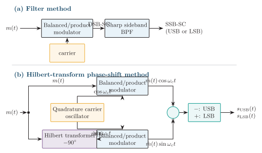
Let $m(t)$ be a real message bandlimited to $|\omega|\leq\Omega_m$ , let $m_a(t)=m(t)+\mathrm{j}\hat{m}(t)$ , and choose $\omega_c>\Omega_m$ so the translated spectra do not overlap. The direct and Hilbert-transform paths modulate quadrature carriers. Their sum or difference produces

The two product-modulator outputs are $I(t)=m(t)\cos\omega_ct$ and $Q(t)=\hat{m}(t)\sin\omega_ct$ . With the convention used here, $I-Q$ selects USB and $I+Q$ selects LSB. the figure also retains the referenced filter-method alternative for comparison.

SSB generation methods. (a) A balanced modulator generates DSB-SC and a sharp BPF selects one sideband. (b) The message is split into direct and Hilbert-transform paths, quadrature product modulators form the two components, and subtraction selects USB while addition selects LSB.

Example — Sideband Cancellation for a Cosine Message

Let $m(t)=\cos\omega_mt$ . With the Hilbert-transform convention adopted above,

\hat m(t)=\sin\omega_mt.

The two balanced-modulator outputs are

\begin{aligned} m(t)\cos\omega_ct &=\cos\omega_mt\cos\omega_ct \\ &=\frac{1}{2}\left[\cos(\omega_c+\omega_m)t +\cos(\omega_c-\omega_m)t\right],\\[3pt] \hat m(t)\sin\omega_ct &=\sin\omega_mt\sin\omega_ct \\ &=\frac{1}{2}\left[\cos(\omega_c-\omega_m)t -\cos(\omega_c+\omega_m)t\right]. \end{aligned}

Therefore subtraction cancels the lower-sideband term and reinforces the upper-sideband term:

\begin{aligned} s_{\mathrm{USB}}(t) &=\cos\omega_mt\cos\omega_ct -\sin\omega_mt\sin\omega_ct \\ &=\boxed{\cos(\omega_c+\omega_m)t}. \end{aligned}

Conversely, addition cancels the upper-sideband term and reinforces the lower-sideband term:

\begin{aligned} s_{\mathrm{LSB}}(t) &=\cos\omega_mt\cos\omega_ct +\sin\omega_mt\sin\omega_ct \\ &=\boxed{\cos(\omega_c-\omega_m)t}. \end{aligned}

The cancellation proof assumes $0<\omega_m<\omega_c$ . By superposition, the same reasoning applies component by component to a general real baseband message.

[!NOTE]

Key Point — Bandwidth and transmitted power

For a message bandlimited to $f_{m(\max)}$ , conventional AM occupies $2f_{m(\max)}$ , whereas SSB occupies only $f_{m(\max)}$ . Thus SSB carries the same information in half the bandwidth. In the ideal suppressed-carrier phase-shift method above, no separate carrier component is transmitted, so carrier power is avoided and the transmitted power is concentrated in the one information-bearing sideband.

Effect of Quadrature Error

Ideal sideband cancellation requires equal path gain and exact quadrature. If the quadrature path has relative gain $g$ and phase error $\epsilon$ , a single-tone model gives desired and residual sideband phasors proportional to $1+ge^{\mathrm{j}\epsilon}$ and $1-ge^{\mathrm{j}\epsilon}$ . Their power ratio is

Perfect gain and phase balance gives infinite ideal rejection. For $g=1$ and small $|\epsilon|$ in radians, $\mathrm{IRR}\approx4/\epsilon^2$ ; even a small phase error therefore leaves a measurable unwanted sideband. Gain ripple and unequal delay have the same practical consequence.

Ideal Phase Shifter and Practical Realization

The Hilbert transformer is often called an ideal $90^\circ$ phase shifter, but this phrase needs two qualifications:

positive and negative frequencies receive opposite phase shifts, as required for a real quadrature output;
the phase shift is frequency independent, but it is not a fixed time delay, whose phase is $-\omega t_d$ .

Its impulse response $h_{\mathrm H}(t)=1/(\pi t)$ is nonzero for $t<0$ and extends infinitely in both directions. It is singular at the origin and not absolutely integrable. Therefore an exact Hilbert transformer is neither causal nor BIBO-stable in the ordinary LTI impulse-response sense, and it cannot be realized physically over all frequencies. This does not contradict the equation: boundedness and energy preservation on $L^2$ are weaker conditions than BIBO stability.

Analog all-pass networks and digital FIR/IIR Hilbert transformers approximate the required phase over a finite band. A causal digital implementation adds delay, so the direct path must receive the same delay to remain aligned with the quadrature path. Finite transition bands, gain ripple, phase error, and delay mismatch limit envelope accuracy and SSB suppression. The discontinuity at DC is another reason no finite causal network can implement the ideal response from zero to infinite frequency.

Exam Traps and Revision Checklist

Exam Focus — Hilbert-transform traps

State the Fourier convention before assigning signs. Here $\mathcal H\{\cos\omega_0t\}=\sin\omega_0t$ and $\mathcal H\{\sin\omega_0t\}=-\cos\omega_0t$ for $\omega_0>0$ .
Do not say every component receives $-90^\circ$ . Positive frequencies receive $-90^\circ$ and negative frequencies receive $+90^\circ$ .
Keep the principal-value symbol in the time-domain definition; the kernel is singular at $\tau=t$ .
Treat DC separately. A constant transforms to zero, $\mathcal H^2x=-x+x_{\mathrm{DC}}$ , and analytic-signal DC is not doubled.
In $X_a(\omega)$ , double positive frequencies and suppress negative frequencies. Omitting the factor of two prevents $\Re\{x_a\}$ from reproducing $x$ .
Equal energy and zero inner product require the stated signal classes. Use power for periodic signals; the zero inner product stated here assumes a real signal.
Interpret $|x_a(t)|$ as a physical envelope only under suitable monocomponent or spectral-separation assumptions. Unwrap phase and do not differentiate through zeros of $x_a(t)$ .
With this convention $I-Q$ gives USB and $I+Q$ gives LSB. Reversing either quadrature phase-shifter polarity interchanges the labels.
An ideal Hilbert transformer is a noncausal, infinite-duration quadrature operator, not a realizable broadband delay line.

[!IMPORTANT]

Key Formula — Core results at a glance

\begin{gathered} \hat{x}(t)=\frac{1}{\pi}\operatorname{PV} \int_{-\infty}^{\infty}\frac{x(\tau)}{t-\tau}\,\mathrm{d}\tau, \qquad \hat{X}(\omega)=-\mathrm{j}\operatorname{sgn}(\omega)X(\omega),\\ x_a(t)=x(t)+\mathrm{j}\hat{x}(t), \qquad X_a(\omega)= \begin{cases} 2X(\omega), & \omega>0,\\ X(0), & \omega=0,\\ 0, & \omega<0, \end{cases}\\ s_{\mathrm{USB}}=m\cos\omega_ct-\hat{m}\sin\omega_ct, \qquad s_{\mathrm{LSB}}=m\cos\omega_ct+\hat{m}\sin\omega_ct. \end{gathered}