Waveguides and Resonant Cavities

Waveguide Fundamentals

Note

Waveguide.

A waveguide is a conducting or dielectric structure that confines and directs electromagnetic waves. Hollow metallic waveguides are used when two-conductor transmission lines become too lossy or impractical at high frequency.

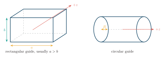
Common waveguide geometries.

Note

Waveguide mode.

A waveguide mode is a distinct electromagnetic field pattern that satisfies Maxwell’s equations and all guide boundary conditions at a particular frequency.

TEM, TE and TM modes. The mode names describe which longitudinal field components vanish relative to the guide axis. The table gives the defining conditions.

Mode type	Longitudinal field condition
TEM	$E_z=0$ and $H_z=0$
TE	$E_z=0$, $H_z\ne0$
TM	$H_z=0$, $E_z\ne0$

Hollow single-conductor waveguides support TE and TM modes, not TEM modes.

A TEM field can be written in terms of an electrostatic potential over the guide cross-section:

$$\mathbf E_t=-\nabla_tV, \qquad \nabla_t^2V=0.$$

The complete wall of a hollow rectangular guide is one connected conductor at one potential. By the uniqueness theorem, the only solution of Laplace’s equation with that boundary value is constant $V$, which would give $\mathbf E_t=0$. A nontrivial TEM mode therefore needs at least two separate conductors at different instantaneous potentials, as in a two-wire or coaxial line.

Feature	Two-wire line	Coaxial line	Hollow waveguide
Conductors	two exposed conductors	inner and outer conductors	one connected wall
Fundamental mode	TEM	TEM	TE or TM
Low-frequency limit	can operate to DC	can operate to DC	has a nonzero cutoff
Shielding	poor	excellent	excellent
Dispersion	ideally nondispersive	ideally nondispersive	dispersive
Typical range	low RF	broad RF range	microwave and high-power RF

Rectangular Waveguide

Note

Rectangular waveguide.

A rectangular waveguide is a hollow conducting guide with rectangular cross-section dimensions $a\times b$, conventionally chosen with $a>b$.

Cutoff frequency. The cutoff frequency $f_{c,mn}$ is the lowest frequency at which mode $(m,n)$ propagates. Below cutoff its axial propagation constant is imaginary and the field is evanescent.

For fields varying as $e^{-j\beta z}$, the longitudinal component $\psi$, equal to $H_z$ for TE modes or $E_z$ for TM modes, satisfies the transverse Helmholtz equation

$$\frac{\partial^2\psi}{\partial x^2} +\frac{\partial^2\psi}{\partial y^2} +k_c^2\psi=0.$$

Separation of variables and the perfect-conductor wall conditions quantize the transverse wavenumbers:

$$k_x=\frac{m\pi}{a}, \qquad k_y=\frac{n\pi}{b}, \qquad k_c^2=k_x^2+k_y^2.$$

The axial propagation constant is

$$\beta^2=\omega^2\mu\varepsilon-k_c^2.$$

At cutoff, $\beta=0$. Substituting $\omega_c=2\pi f_c$ therefore gives

$$f_{c,mn}=\frac{1}{2\sqrt{\mu\varepsilon}} \sqrt{\left(\frac{m}{a}\right)^2+\left(\frac{n}{b}\right)^2}.$$

For TE modes, $m$ and $n$ may individually be zero but not both. For TM modes, both indices must be nonzero. Above cutoff $\beta$ is real and the mode propagates; below cutoff it is imaginary and the mode is evanescent.

Note

Dominant waveguide mode.

The dominant mode is the propagating mode with the lowest cutoff frequency. For a rectangular waveguide with $a>b$, it is $\mathrm{TE}_{10}$.

$$f_{c,10}=\frac{1}{2a\sqrt{\mu\varepsilon}}.$$

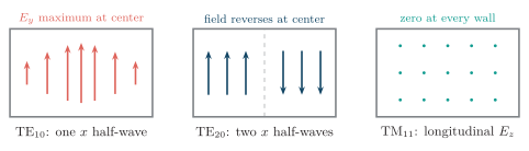
Rectangular waveguide mode patterns.

Note

Guide wavelength and velocities.

Guide wavelength $\lambda_g$ is the axial distance over which phase changes by $2\pi$; phase velocity $v_p$ is the speed of a constant-phase point; group velocity $v_g$ is the speed of the wave envelope and energy in a lossless guide.

For operation above cutoff,

$$\lambda_g=\frac{\lambda}{\sqrt{1-(f_c/f)^2}},$$ $$v_p=\frac{v}{\sqrt{1-(f_c/f)^2}}, \qquad v_g=v\sqrt{1-(f_c/f)^2}.$$

Note

Wave impedance.

Wave impedance is the ratio of transverse electric-field magnitude to transverse magnetic-field magnitude for a specified mode.

For TE and TM modes,

$$Z_{\text{TE}}=\frac{\eta}{\sqrt{1-(f_c/f)^2}}, \qquad Z_{\text{TM}}=\eta\sqrt{1-(f_c/f)^2}.$$

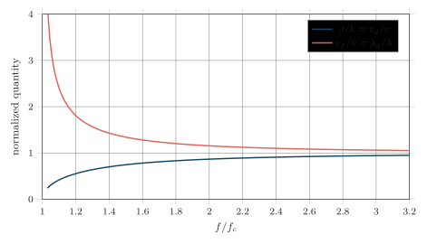
Waveguide dispersion above cutoff.

Circular Waveguide

Note

Circular waveguide.

A circular waveguide is a hollow conducting guide with a circular cross-section; its cutoff frequencies are determined by roots of Bessel functions and their derivatives.

Dominant circular-waveguide mode. The lowest-cutoff mode of a hollow circular guide is normally $\mathrm{TE}_{11}$.

Key quantities are cutoff frequency, dominant mode, guide wavelength, phase velocity, group velocity and wave impedance.

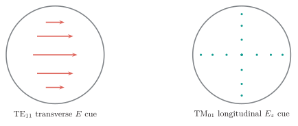
Circular waveguide mode cues.

Resonant Cavities

Note

Resonant cavity.

A resonant cavity is a closed conducting enclosure in which electromagnetic energy is stored in discrete standing-wave modes. It is the microwave equivalent of a lumped $LC$ resonator.

At low frequency, inductors and capacitors can be treated as separate lumped elements. At microwave frequency, their dimensions may become comparable with wavelength, conductor loss increases, and stray reactances become important. A metallic cavity instead uses distributed electric and magnetic fields:

• electric-field energy acts like energy stored in a capacitor;

• magnetic-field energy acts like energy stored in an inductor;

• wall and dielectric losses act like resistance;

• only discrete field patterns and resonant frequencies satisfy all boundary conditions.

Formation from a Waveguide

Consider a uniform waveguide carrying a TE or TM mode. Closing it with perfect electric conductor (PEC) plates at $z=0$ and $z=d$ causes complete reflection. The forward and reflected waves combine to form a standing wave.

Note

Standing wave.

A standing wave is the stationary field pattern formed by superposition of equal-frequency waves travelling in opposite directions; it has fixed nodes and antinodes.

Perfect electric conductor. A perfect electric conductor (PEC) is an ideal material of infinite conductivity with zero internal electric field. At its surface, tangential electric field and normal magnetic flux density vanish.

At a PEC wall,

$$\hat{\mathbf n}\times\mathbf E=0, \qquad \hat{\mathbf n}\cdot\mathbf B=0.$$

Thus the tangential electric field must vanish on every cavity wall. Surface charge supports a normal electric field, while surface current supports a tangential magnetic field.

For the end plates to coincide with standing-wave electric-field nodes, the axial phase condition is

$$\beta_zd=p\pi, \qquad p=1,2,3,\ldots$$

or

$$\boxed{d=\frac{p\lambda_g}{2}},$$

where

$$\lambda_g=\frac{2\pi}{\beta_z}$$

is the guide wavelength of that mode. The cavity length must contain an integer number of guide half-wavelengths, not generally free-space half-wavelengths.

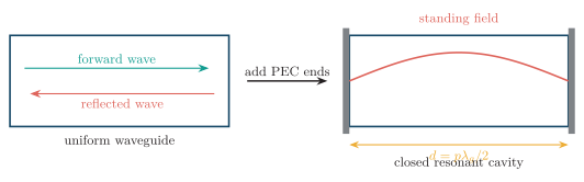
Shorted waveguide as a cavity.

How to read the figure. The left-hand guide supports separate forward and reflected travelling waves. Adding PEC end plates forces repeated reflection and fixes electric-field nodes at the ends. On the right, the two waves have combined into a standing field. Only frequencies satisfying $d=p\lambda_g/2$ reproduce the same phase after a round trip and build to a large amplitude.

There is no net time-average power flow through a lossless closed cavity. Energy remains stored and moves back and forth between electric and magnetic forms.

Rectangular-Cavity Resonance

Take a homogeneous rectangular cavity with dimensions

$$0<x<a, \qquad 0<y<b, \qquad 0<z<d,$$

filled with a medium of permeability $\mu$ and permittivity $\varepsilon$. Define

$$v=\frac{1}{\sqrt{\mu\varepsilon}}, \qquad k=\omega\sqrt{\mu\varepsilon}.$$

For the corresponding rectangular waveguide,

$$k_c^2= \left(\frac{m\pi}{a}\right)^2 +\left(\frac{n\pi}{b}\right)^2$$

and

$$\beta_z^2=k^2-k_c^2.$$

The end plates require

$$\beta_z=\frac{p\pi}{d}.$$

Substitution gives the cavity eigenvalue equation

$$k^2= \left(\frac{m\pi}{a}\right)^2 +\left(\frac{n\pi}{b}\right)^2 +\left(\frac{p\pi}{d}\right)^2.$$

Note

Cavity resonant frequency.

A cavity resonant frequency, or eigenfrequency, is a discrete frequency at which a non-zero field pattern satisfies Maxwell’s equations and every conducting-wall boundary condition.

Therefore the resonant angular frequency is

$$\omega_{mnp}= \frac{\pi}{\sqrt{\mu\varepsilon}} \sqrt{ \left(\frac{m}{a}\right)^2 +\left(\frac{n}{b}\right)^2 +\left(\frac{p}{d}\right)^2 },$$

and the resonant frequency is

$$\boxed{ f_{mnp}= \frac{1}{2\sqrt{\mu\varepsilon}} \sqrt{ \left(\frac{m}{a}\right)^2 +\left(\frac{n}{b}\right)^2 +\left(\frac{p}{d}\right)^2 } }.$$

For an air-filled cavity,

$$f_{mnp}= \frac{c}{2} \sqrt{ \left(\frac{m}{a}\right)^2 +\left(\frac{n}{b}\right)^2 +\left(\frac{p}{d}\right)^2 }.$$

Note

Cavity mode indices and degeneracy.

The integers $m$, $n$ and $p$ identify field variations along $x$, $y$ and $z$. Modes with different index sets but the same resonant frequency are degenerate modes.

TE and TM Cavity Modes

Note

TE and TM cavity modes.

Relative to the chosen longitudinal $z$ direction, a TE mode has $E_z=0$ and $H_z\ne0$, whereas a TM mode has $H_z=0$ and $E_z\ne0$. The table also gives the allowed cavity indices.

Mode	Longitudinal field	Allowed indices
$\mathrm{TE}_{mnp}$	$E_z=0$, $H_z\ne0$	$m,n=0,1,2,\ldots$, but not both zero; $p=1,2,\ldots$
$\mathrm{TM}_{mnp}$	$H_z=0$, $E_z\ne0$	$m,n=1,2,\ldots$; $p=0,1,2,\ldots$

There is no non-zero $\mathrm{TE}_{00p}$ field, and $\mathrm{TM}$ modes cannot have $m=0$ or $n=0$. Unlike an ordinary propagating-wave condition, $p=0$ is allowed for TM modes because $E_z$ is normal to the end plates and need not vanish there.

Representative longitudinal field functions are

$$H_z=H_0 \cos\left(\frac{m\pi x}{a}\right) \cos\left(\frac{n\pi y}{b}\right) \sin\left(\frac{p\pi z}{d}\right)$$

for TE modes, and

$$E_z=E_0 \sin\left(\frac{m\pi x}{a}\right) \sin\left(\frac{n\pi y}{b}\right) \cos\left(\frac{p\pi z}{d}\right)$$

for TM modes. The remaining components follow from Maxwell’s curl equations.

Important examples are

$$f_{101}^{\mathrm{TE}} =\frac{v}{2} \sqrt{\frac{1}{a^2}+\frac{1}{d^2}}$$

and

$$f_{110}^{\mathrm{TM}} =\frac{v}{2} \sqrt{\frac{1}{a^2}+\frac{1}{b^2}}.$$

Note

Dominant cavity mode.

The dominant cavity mode is the permitted mode with the lowest resonant frequency. It depends on $a$, $b$ and $d$; unlike a standard rectangular waveguide, a cavity has no universal dominant mode. For many cavities with $a>b$ and $d>b$, $\mathrm{TE}_{101}$ is the lowest mode.

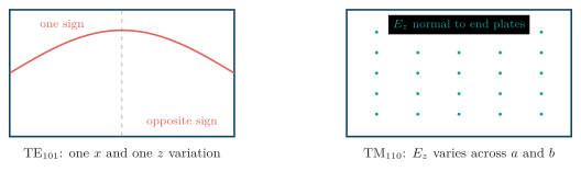
Cavity mode cues.

How to read the figure. The left panel is a qualitative $x$-$z$ cut of $\mathrm{TE}_{101}$. The field changes once across $x$ and once along $z$, and opposite signs indicate a $180^\circ$ phase reversal across a node. The right panel shows $\mathrm{TM}_{110}$ in an $x$-$y$ cut. The dots represent $E_z$ normal to the page and to the end plates; it varies across both $a$ and $b$ but has no axial variation because $p=0$.

Stored Energy and the Resonance Process

Note

Stored electric and magnetic energy.

Stored electric energy $W_e$ is the volume integral of electric energy density, and stored magnetic energy $W_m$ is the corresponding integral of magnetic energy density. With peak-value phasors, each density carries a factor of $1/4$.

The cycle-average energies are

$$W_e=\frac{1}{4}\iiint_V \varepsilon|\mathbf E|^2\,dV$$

and

$$W_m=\frac{1}{4}\iiint_V \mu|\mathbf H|^2\,dV.$$

At resonance in a lossless cavity,

$$\boxed{W_e=W_m},$$

and the total cycle-average stored energy is

$$W=W_e+W_m.$$

The equality refers to cycle-average energies. Instantaneously, electric and magnetic energy exchange every quarter-cycle:

1. At an electric-field maximum, energy is mainly electric and the magnetic field is momentarily minimum.

2. One quarter-cycle later, energy is mainly magnetic.

3. Another quarter-cycle later, the electric field is maximum with reversed polarity.

4. The process repeats, analogous to energy exchange between $C$ and $L$ in an ideal resonator.

Near a single isolated mode, a cavity can be represented by an equivalent RLC resonator with

$$\omega_0=\frac{1}{\sqrt{LC}}.$$

The equivalent circuit is a local model near resonance; the distributed cavity can support many separate modes, each with its own equivalent resonant branch.

Cavity Losses

An ideal PEC cavity would store energy forever and have infinite quality factor. A real cavity loses energy through several mechanisms.

Conductor loss

Finite wall conductivity causes surface-current heating.

Note

Surface resistance and skin depth.

Surface resistance $R_s$ is the effective RF resistance of one square of a good conductor’s surface. Skin depth $\delta_s$ is the depth at which field amplitude falls to $1/e$ of its surface value.

At high frequency,

$$R_s=\sqrt{\frac{\omega\mu_c}{2\sigma}} =\frac{1}{\sigma\delta_s},$$

where

$$\delta_s=\sqrt{\frac{2}{\omega\mu_c\sigma}}$$

is skin depth. For peak-value phasors, conductor power loss is

$$P_c=\frac{R_s}{2} \iint_S|\mathbf H_t|^2\,dS.$$

Conductor loss is strongest where tangential magnetic field, and therefore wall surface current, is large.

Dielectric loss

Note

Dielectric loss tangent.

Loss tangent $\tan\delta$ is the ratio of the lossy to energy-storing parts of a dielectric response; for a low-loss dielectric it is approximately the reciprocal of dielectric quality factor.

For a dielectric with loss tangent $\tan\delta$, the time-average loss is

$$P_d=\frac{\omega\varepsilon'\tan\delta}{2} \iiint_V|\mathbf E|^2\,dV.$$

For a uniformly filled low-loss cavity,

$$Q_d\approx\frac{1}{\tan\delta}.$$

External and radiation loss

Energy also leaves through coupling probes, loops, apertures, imperfect joints and leakage. External coupling is intentional when power must enter or leave the cavity, but it lowers the measured or loaded quality factor.

Quality Factor

Note

Quality factor.

Quality factor $Q$ measures stored energy relative to energy lost per radian at resonance. A higher $Q$ means lower loss, slower decay and narrower bandwidth.

$$\boxed{ Q=\omega_0\frac{W}{P_{\mathrm{loss}}} }.$$

Equivalently,

$$Q=2\pi \frac{\mathrm{energy\ stored}} {\mathrm{energy\ lost\ per\ cycle}}.$$

A high-$Q$ cavity has low loss, slow field decay, a sharp resonance and narrow bandwidth.

Unloaded, external and loaded quality factors

Note

Cavity quality factors.

Unloaded $Q_0$ includes internal losses only, external $Q_e$ represents power extracted through coupling, and loaded $Q_L$ includes both internal and external losses. The table separates the individual terms.

Symbol	Meaning
$Q_c$	limitation from conducting-wall loss
$Q_d$	limitation from dielectric loss
$Q_0$	unloaded $Q$ due to all internal losses
$Q_e$	external $Q$ due to energy extracted by coupling
$Q_L$	loaded $Q$ including internal and external losses

Internal loss mechanisms combine as

$$\frac{1}{Q_0}=\frac{1}{Q_c}+\frac{1}{Q_d}+\frac{1}{Q_{\mathrm{other}}}.$$

For one external coupling port,

$$\boxed{ \frac{1}{Q_L}=\frac{1}{Q_0}+\frac{1}{Q_e} }.$$

Note

Coupling coefficient.

The cavity coupling coefficient $\beta_c$ is the ratio $Q_0/Q_e$ and compares external loading with internal loss.

$$\beta_c=\frac{Q_0}{Q_e},$$

so

$$Q_L=\frac{Q_0}{1+\beta_c}.$$

Coupling	Condition	Interpretation
Undercoupled	$\beta_c<1$	internal loss exceeds extracted power
Critically coupled	$\beta_c=1$	internal and external losses are equal
Overcoupled	$\beta_c>1$	external loading dominates

Note

Coupling regimes.

A cavity is undercoupled when internal loss dominates, critically coupled when internal and external losses are equal, and overcoupled when external loading dominates.

At critical coupling, $Q_e=Q_0$ and $Q_L=Q_0/2$.

If the source is removed, stored energy decays approximately as

$$W(t)=W(0)e^{-\omega_0t/Q_L},$$

while field amplitude decays as

$$|E(t)|\mathrel{\propto} e^{-\omega_0t/(2Q_L)}.$$

Resonance Curve and Bandwidth

For a lightly damped single resonance, the normalized power response near $f_0$ is approximately

$$\frac{P(f)}{P_{\max}} \approx \frac{1}{1+ 4Q_L^2\left(\dfrac{f-f_0}{f_0}\right)^2}.$$

Note

Half-power frequencies and bandwidth.

The lower and upper half-power frequencies $f_1$ and $f_2$ are the points where power is one half of its resonant maximum. Their difference $\Delta f=f_2-f_1$ is the half-power, or $-3$ dB, bandwidth.

At these points,

$$P(f_1)=P(f_2)=\frac{P_{\max}}{2},$$

which is $-3.01$ dB relative to the peak. The half-power bandwidth is

$$\Delta f=f_2-f_1.$$

For $Q_L\gg1$,

$$\boxed{ Q_L=\frac{f_0}{\Delta f} }.$$

Thus a larger $Q_L$ produces a narrower resonance curve.

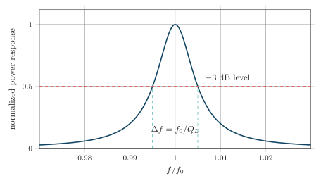
Resonance curve and bandwidth.

How to read the figure. The horizontal axis is frequency normalized to the resonant frequency, so the peak occurs at $f/f_0=1$. The cyan dashed line is half the peak power, or $-3$ dB. Its two intersections with the response define $f_1$ and $f_2$. The illustrated curve has $Q_L=100$, so $\Delta f/f_0=1/100=0.01$ and the half-power points lie approximately at $0.995f_0$ and $1.005f_0$.

Excitation and Coupling

A cavity mode is excited efficiently only when the source has the correct field type, orientation and position. Placing a coupler at a field node gives little coupling even when the frequency is correct.

Electric-probe coupling

Note

Electric-probe coupling.

Electric-probe coupling uses a short conducting probe as a small electric dipole to exchange energy with a cavity’s electric field.

• Place it near an electric-field maximum.

• Align it parallel to the desired electric-field component.

• Probe length and insertion depth control coupling strength.

Magnetic-loop coupling

Note

Magnetic-loop coupling.

Magnetic-loop coupling uses a small conducting loop to exchange energy through magnetic flux linking the loop.

• Place it near a magnetic-field maximum.

• Orient its plane so the desired magnetic field passes through the loop.

• Loop area and rotation control coupling strength.

Aperture or iris coupling

Note

Aperture coupling.

Aperture, or iris, coupling transfers electromagnetic energy through an opening in the common wall between a waveguide and a cavity.

• Position the aperture where the required waveguide and cavity fields overlap strongly.

• Aperture size and shape control coupling.

• Small apertures weakly perturb the cavity; a large iris increases loading and can shift the resonant frequency.

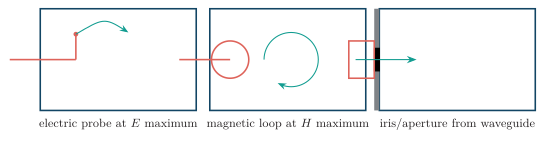
Cavity coupling methods.

How to read the figure. The left sketch places an electric probe at an $E$-field maximum and aligns it with the field. The centre sketch places a loop where $H$ is large so magnetic flux links the loop. The right sketch uses an iris in a shared waveguide wall; the travelling guide mode transfers power through the opening to the matching cavity mode.

Selective excitation is possible because orthogonal cavity modes have different field symmetries. A centrally placed probe may excite one mode strongly while giving zero coupling to another mode whose electric field has a node there.

Tuning a Cavity

Resonant frequency changes when cavity dimensions or material properties change:

$$f_0\mathrel{\propto}\frac{1}{\sqrt{\mu\varepsilon}}.$$

Common tuning methods are

• moving a conducting wall or plunger to change effective cavity dimensions;

• inserting a metallic tuning screw where electric field is strong;

• inserting dielectric material to increase effective permittivity and generally lower frequency;

• changing temperature, which changes dimensions, conductivity and material properties.

A tuner also perturbs the field and can alter $Q$, coupling and nearby-mode separation.

Waveguide and Cavity Comparison

Property	Uniform waveguide	Resonant cavity
Structure	open or terminated transmission path	closed conducting enclosure
Frequency condition	any $f>f_c$ can propagate	only discrete $f_{mnp}$ resonate strongly
Axial field	travelling wave is possible	standing wave
Average power flow	carries power along the guide	ideally zero through the closed cavity
Main use	transfer microwave power	store energy and select frequency

Applications

Resonant cavities are used in

• microwave oscillators such as klystrons and magnetrons;

• narrowband filters, duplexers and frequency-selective networks;

• wavemeters and frequency standards;

• radar and satellite communication equipment;

• particle accelerators, where resonant electric fields accelerate charged particles;

• electron-spin and nuclear-magnetic-resonance systems;

• measurement of dielectric constant, loss tangent and surface resistance;

• microwave heating and industrial processing.

Worked Examples

Rectangular-waveguide cutoff frequency

For an air-filled rectangular waveguide with broad dimension $a=4\ \mathrm{cm}=0.04\ \mathrm m$, the dominant-mode cutoff is

$$f_{c,10}=\frac{c}{2a} =\frac{3.00\times10^8}{2(0.04)} =\boxed{3.75\ \mathrm{GHz}}.$$

Below this frequency the $\mathrm{TE}_{10}$ field is evanescent. Practical single-mode operation must be above this cutoff and below the cutoff of the next mode.

Rectangular-cavity resonant frequency

An air-filled cavity has

$$a=4\ \mathrm{cm}, \qquad b=2\ \mathrm{cm}, \qquad d=5\ \mathrm{cm}.$$

Find the $\mathrm{TE}_{101}$ resonant frequency.

For $m=1$, $n=0$ and $p=1$,

$$f_{101}=\frac{c}{2} \sqrt{\frac{1}{a^2}+\frac{1}{d^2}}.$$

Substituting SI values,

$$f_{101}=\frac{3\times10^8}{2} \sqrt{ \frac{1}{(0.04)^2} +\frac{1}{(0.05)^2} }.$$

Therefore,

$$\boxed{f_{101}\approx4.80\ \mathrm{GHz}}.$$

The dimension $b$ does not appear because $n=0$ for this TE mode.

Bandwidth from loaded quality factor

A cavity resonates at $f_0=10$ GHz and has $Q_L=2000$. Its half-power bandwidth is

$$\Delta f=\frac{f_0}{Q_L} =\frac{10\times10^9}{2000} =5\times10^6\ \mathrm{Hz}.$$

Hence

$$\boxed{\Delta f=5\ \mathrm{MHz}}.$$

For a symmetric high-$Q$ response, the half-power frequencies are approximately

$$f_1=9.9975\ \mathrm{GHz}, \qquad f_2=10.0025\ \mathrm{GHz}.$$

Loaded quality factor under critical coupling

If an unloaded cavity has $Q_0=6000$ and is critically coupled, then

$$Q_e=Q_0=6000$$

and

$$Q_L=\frac{Q_0}{1+\beta_c} =\frac{6000}{2} =3000.$$

Chapter Summary

1. A cavity is a waveguide or conducting enclosure closed in all directions.

2. PEC walls require zero tangential electric field and create standing waves.

3. A rectangular cavity resonates at

$$f_{mnp}=\frac{1}{2\sqrt{\mu\varepsilon}} \sqrt{ \left(\frac{m}{a}\right)^2 +\left(\frac{n}{b}\right)^2 +\left(\frac{p}{d}\right)^2 }.$$

1. TE modes have $E_z=0$; TM modes have $H_z=0$.

2. Electric and magnetic energies exchange every quarter-cycle and have equal cycle averages at resonance.

3. Quality factor is $Q=\omega_0W/P_{\mathrm{loss}}$.

4. Loaded half-power bandwidth is $\Delta f=f_0/Q_L$.

5. Electric probes, magnetic loops and apertures couple to the corresponding field maxima.

Interpretive Cautions

• Using free-space wavelength in $d=p\lambda_g/2$ instead of guide wavelength.

• Calling $\mathrm{TE}_{100}$ a valid closed-cavity mode; TE modes require $p\ge1$ when $z$ is the closed-guide axis.

• Rejecting $\mathrm{TM}_{110}$ because $p=0$; zero axial variation is allowed for TM modes.

• Assuming $E_n=0$ at a PEC wall. Only tangential $E$ must be zero; normal $E$ can be supported by surface charge.

• Using unloaded $Q_0$ in a measured bandwidth relation. The observed bandwidth gives loaded $Q_L$.