Energy, Power, and Autocorrelation

Energy and Power Signal Recap

the section gives the full continuous- and discrete-time definitions and classification examples. The decisive tests are recalled here because the correct correlation definition depends on the signal class:

Caution

Key Formula — Energy and power classification

$$0<E_x<\infty\ \Longrightarrow\ P_x=0 \quad\text{(energy signal)},$$$$0<P_x<\infty\ \Longrightarrow\ E_x=\infty \quad\text{(power signal)}.$$

A nonzero signal cannot belong to both classes. Some signals belong to neither, and the all-zero signal is normally excluded by the strict positive conditions. For periodic signals whose squared magnitude is integrable or summable over one period,

Caution

Key Formula — Average power over one period

$$P_x=\frac{1}{T_0}\int_{t_0}^{t_0+T_0}|x(t)|^2\,\mathrm{d}t, \qquad P_x=\frac{1}{N_0}\sum_{n=n_0}^{n_0+N_0-1}|x[n]|^2.$$

The starting point is arbitrary because a complete period is averaged.

Energy and Power Spectral Density

For the angular-frequency Fourier convention used in this chapter, a CT energy signal with transform $X(\omega)$ has energy spectral density (ESD)

Caution

Key Formula — Continuous-time energy spectral density

$$\Psi_x(\omega)=|X(\omega)|^2, \qquad E_x=\frac{1}{2\pi}\int_{-\infty}^{\infty} \Psi_x(\omega)\,\mathrm{d}\omega.$$

For a DT energy signal with DTFT $X(e^{\mathrm{j}\Omega})$,

$$\Psi_x(e^{\mathrm{j}\Omega})=|X(e^{\mathrm{j}\Omega})|^2, \qquad E_x=\frac{1}{2\pi}\int_{-\pi}^{\pi} \Psi_x(e^{\mathrm{j}\Omega})\,\mathrm{d}\Omega.$$

ESD therefore states where a finite total energy lies in frequency.

A power signal generally has infinite total energy, so its ordinary Fourier transform cannot simply be squared as a finite-energy function. Its power spectral density (PSD) is instead defined through autocorrelation. Under the same angular-frequency convention,

Caution

Key Formula — Power recovered from PSD

$$P_x=R_{xx}(0) =\frac{1}{2\pi}\int_{-\infty}^{\infty}S_{xx}(\omega)\,\mathrm{d}\omega,$$

with an integral over any $2\pi$ interval for a DT PSD. ESD has units of energy per unit frequency and integrates to energy; PSD has units of mean-square value per unit frequency and integrates to average power.

Periodic power signals have line spectra. If $x(t)=\sum_{r=-\infty}^{\infty}C_r e^{\mathrm{j}r\omega_0t}$, then

Caution

Key Formula — PSD of a periodic deterministic signal

$$S_{xx}(\omega)=2\pi\sum_{r=-\infty}^{\infty} |C_r|^2\delta(\omega-r\omega_0), \qquad P_x=\sum_{r=-\infty}^{\infty}|C_r|^2.$$

This is the power-signal counterpart of Parseval’s theorem.

Deterministic Autocorrelation

Autocorrelation measures similarity between a signal and a delayed copy of itself. This section consistently uses the lag convention $x^*(t-\tau)$ or $x^*[n-m]$.

Energy Signals

For CT and DT energy signals,

Note

Law — Energy-signal autocorrelation

$$\begin{aligned} R_{xx}(\tau) &=\int_{-\infty}^{\infty}x(t)x^*(t-\tau)\,\mathrm{d}t,\\ R_{xx}[m] &=\sum_{n=-\infty}^{\infty}x[n]x^*[n-m]. \end{aligned}$$

These are inner products between the signal and a shifted version. For real signals the conjugate has no visible effect, but it must be retained for complex baseband signals.

Power Signals

For deterministic power signals, replace total integration or summation by a long-time average:

Note

Law — Power-signal autocorrelation

$$\begin{aligned} R_{xx}(\tau) &=\lim_{T\to\infty}\frac{1}{2T} \int_{-T}^{T}x(t)x^*(t-\tau)\,\mathrm{d}t,\\ R_{xx}[m] &=\lim_{N\to\infty}\frac{1}{2N+1} \sum_{n=-N}^{N}x[n]x^*[n-m], \end{aligned}$$

provided the limits exist. For a CT periodic signal, the equivalent one-period expression is

$$R_{xx}(\tau)=\frac{1}{T_0} \int_{t_0}^{t_0+T_0}x(t)x^*(t-\tau)\,\mathrm{d}t.$$

The DT periodic formula similarly averages over one complete period.

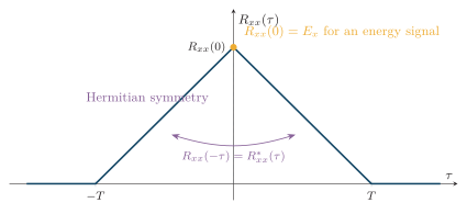
A typical real finite-pulse autocorrelation. It is even, reaches its maximum magnitude at zero lag, and has $R_{xx}(0)$ equal to signal energy. Other signals need not have this triangular shape.

Random-Process Autocorrelation

For a complex random process $X(t)$, the general second-order correlation is

$$R_X(t_1,t_2)=\mathbb{E}\!\left\{X(t_1)X^*(t_2)\right\}.$$

If the process is wide-sense stationary (WSS), its mean is constant and its correlation depends only on the lag $\tau=t_1-t_2$:

Caution

Key Formula — WSS autocorrelation

$$R_X(\tau)=\mathbb{E}\!\left\{X(t)X^*(t-\tau)\right\}, \qquad R_X[m]=\mathbb{E}\!\left\{X[n]X^*[n-m]\right\}.$$

Expectation is an ensemble average. A time average from one realization equals it only under an appropriate ergodicity assumption; stationarity by itself does not guarantee that equality.

Autocorrelation must also be distinguished from autocovariance. If the WSS mean is $\mu_X$, then

$$C_X(\tau)=R_X(\tau)-|\mu_X|^2.$$

Thus $R_X(0)=\mathbb{E}\{|X(t)|^2\}$ is mean square, not variance unless the mean is zero. A nonzero mean creates a constant floor in autocorrelation and a DC spectral line in the PSD; mean removal is often necessary before estimating periodicity or delay.

Autocorrelation Properties

The following properties hold when the defining energy, time-average power, or WSS second moment exists.

1. Value at zero: Zero lag equals the relevant signal measure:

$$R_{xx}(0)=E_x\quad\text{for an energy signal}, \qquad R_{xx}(0)=P_x\quad\text{for a power signal}.$$

The DT statements use $R_{xx}[0]$; for a WSS process it is the mean-square value.

2. Hermitian symmetry: Autocorrelation obeys

$$R_{xx}(-\tau)=R_{xx}^*(\tau), \qquad R_{xx}[-m]=R_{xx}^*[m].$$

It is real and even for a real signal. For a complex signal it need not be real or even; its real part is even and its imaginary part is odd.

3. Maximum magnitude at zero: Cauchy–Schwarz gives

$$|R_{xx}(\tau)|\leq R_{xx}(0), \qquad |R_{xx}[m]|\leq R_{xx}[0].$$

This is a magnitude bound, not an ordering of complex values. Equality can also occur at a nonzero lag when a shifted signal is proportional to the original, as for periodic signals; zero lag need not be the unique peak.

4. Periodicity: If $x(t)$ has period $T_0$, then $R_{xx}(\tau)$ is also periodic with period $T_0$. The analogous statement holds for a DT period $N_0$.

5. Nonnegative definiteness: For arbitrary complex constants $c_i$ and lags $\tau_i$,

$$\sum_i\sum_j c_i c_j^*R_{xx}(\tau_i-\tau_j)\geq0.$$

An autocorrelation may still take negative pointwise values; this condition is what guarantees a nonnegative PSD.

6. Ideal white noise: A zero-mean ideal white-noise process has

$$R_{ww}(\tau)=\frac{N_0}{2}\delta(\tau), \qquad R_{ww}[m]=\sigma_w^2\delta[m].$$

Distinct lags are uncorrelated. The impulse correlation and flat infinite-bandwidth PSD describe an idealization, not every random process; physical white noise is bandwidth-limited.

Wiener–Khinchin Theorem

The Fourier transform of autocorrelation gives spectral density. For a CT energy signal this is the ESD; for a deterministic power signal or WSS random process it is the PSD:

Note

Law — Continuous-time Wiener–Khinchin relation

$$S_{xx}(\omega) =\int_{-\infty}^{\infty}R_{xx}(\tau)e^{-\mathrm{j}\omega\tau}\,\mathrm{d}\tau, \qquad R_{xx}(\tau) =\frac{1}{2\pi}\int_{-\infty}^{\infty} S_{xx}(\omega)e^{\mathrm{j}\omega\tau}\,\mathrm{d}\omega.$$

For an energy signal, direct substitution gives

$$S_{xx}(\omega)=|X(\omega)|^2.$$

The DT counterpart is the Fourier-series pair

Caution

Key Formula — Discrete-time Wiener–Khinchin relation

$$S_{xx}(e^{\mathrm{j}\Omega}) =\sum_{m=-\infty}^{\infty}R_{xx}[m]e^{-\mathrm{j}\Omega m}, \qquad R_{xx}[m] =\frac{1}{2\pi}\int_{-\pi}^{\pi} S_{xx}(e^{\mathrm{j}\Omega})e^{\mathrm{j}\Omega m}\,\mathrm{d}\Omega.$$

The PSD is real and nonnegative. Setting lag to zero recovers total energy or average power by integrating the applicable density.

For a finite $N$-sample record, define circular autocorrelation by

$$r_{xx}^{(c)}[m]=\sum_{n=0}^{N-1}x[n]x^*[(n-m)_N].$$

It obeys the exact DFT pair

$$r_{xx}^{(c)}[m]\longleftrightarrow |X[k]|^2.$$

An FFT and IFFT therefore compute circular correlation efficiently. Linear correlation requires sufficient zero padding to prevent wraparound, exactly as for linear convolution.

Cross-Correlation and Cross-Spectral Density

Cross-correlation compares two different signals. For CT and DT energy signals,

Caution

Key Formula — Cross-correlation

$$\begin{aligned} R_{xy}(\tau) &=\int_{-\infty}^{\infty}x(t)y^*(t-\tau)\,\mathrm{d}t,\\ R_{xy}[m] &=\sum_{n=-\infty}^{\infty}x[n]y^*[n-m]. \end{aligned}$$

Power-signal versions use time averages. Jointly WSS random processes use the ensemble correlation

$$R_{XY}(\tau)=\mathbb{E}\!\left\{X(t)Y^*(t-\tau)\right\}.$$

Unlike autocorrelation, cross-correlation is generally neither even nor real:

Caution

Key Formula — Cross-correlation reciprocity

$$R_{xy}(\tau)=R_{yx}^*(-\tau), \qquad R_{xy}[m]=R_{yx}^*[-m].$$

Its Fourier transform is the cross-spectral density $S_{xy}(\omega)=\mathcal{F}\{R_{xy}(\tau)\}$; for energy signals, $S_{xy}(\omega)=X(\omega)Y^*(\omega)$.

The correlation peak locates relative delay, but its sign depends on order and lag convention. With the convention used here, if $y(t)=x(t-\tau_0)$, then $R_{xy}(\tau)$ peaks at $-\tau_0$, while $R_{yx}(\tau)$ peaks at $+\tau_0$.

Correlation versus Convolution

Correlation is convolution with a conjugated, time-reversed second signal:

Note

Law — Correlation as convolution

$$R_{xy}(\tau)=\bigl[x*y^*(-\mathord{\cdot})\bigr](\tau), \qquad R_{xy}[m]=\bigl[x*y^*[-\mathord{\cdot}]\bigr][m].$$

Thus the same direct or FFT-based convolution routine can compute correlation after conjugate reversal of one input.

Normalized Correlation

For finite, nonzero signal energies, a dimensionless coefficient is

$$\rho_{xy}(\tau)=\frac{R_{xy}(\tau)}{\sqrt{E_xE_y}}, \qquad |\rho_{xy}(\tau)|\leq1.$$

For power signals or WSS processes, replace $E_x,E_y$ by the corresponding zero-lag mean-square values. Several practical qualifications matter:

• subtract sample means when the aim is waveform similarity rather than a shared DC level;

• for finite records, use lag-dependent norms over the samples that actually overlap, or explicitly accept edge bias from a fixed denominator;

• the peak may repeat for periodic data and may broaden or move because of filtering, noise, or multipath;

• normalization is undefined when either denominator is zero, and high correlation alone does not establish causation.

Autocorrelation of a Sinusoid

Note

Example — Autocorrelation of a Sinusoidal Power Signal

Let

$$x(t)=A\cos(\omega_0t+\phi),$$

with real $A$ and $\omega_0\neq0$. Averaging over one period and applying the product-to-sum identity gives

$$\begin{aligned} R_{xx}(\tau) &=\frac{1}{T_0}\int_0^{T_0} A\cos(\omega_0t+\phi) A\cos(\omega_0(t-\tau)+\phi)\,\mathrm{d}t\\ &=\boxed{\frac{A^2}{2}\cos(\omega_0\tau)}. \end{aligned}$$

At zero lag, $R_{xx}(0)=A^2/2$, exactly the sinusoid’s average power. The phase $\phi$ disappears under time averaging, and the periodic correlation has equal peaks at integer multiples of $T_0$. Its two-sided PSD is

$$S_{xx}(\omega)=\frac{\pi A^2}{2} \bigl[\delta(\omega-\omega_0)+\delta(\omega+\omega_0)\bigr].$$

Autocorrelation can therefore reveal unknown periodicity even when the sinusoid is embedded in noise.

Uses and Quick Review

Autocorrelation detects hidden periodicity, estimates pitch and symbol or clock timing, and converts naturally to PSD. Cross-correlation estimates relative delay and similarity in radar and sonar ranging, communication synchronization, matched filtering, channel sounding, and pattern matching.

Tip

Exam Focus — Correlation Quick Review

• Signal class: Energy signals use total correlation integrals or sums; power signals use time averages; WSS processes use ensemble averages.

• Zero and symmetry: $R_{xx}(0)$ equals energy, power, or mean square, and $R_{xx}(-\tau)=R_{xx}^*(\tau)$.

• Peak condition: $|R_{xx}(\tau)|\leq R_{xx}(0)$, but periodic or proportional shifts can produce additional equal peaks.

• Wiener–Khinchin: Autocorrelation and ESD or PSD form a Fourier pair; ideal white noise has impulse correlation and flat PSD.

• Cross-correlation: $R_{xy}=R_{yx}^*(-\tau)$ and equals convolution with a conjugate-reversed second signal.