Circular Convolution

Definition and Modulo Indexing

For two $N$ -point sequences $x[n]$ and $h[n]$ , their $N$ -point circular convolution is

where $(n-m)_N$ denotes the residue of $n-m$ modulo $N$ . For example, with $N=4$ , an index of $-1$ is read as $3$ and an index of $5$ is read as $1$ .

Modulo indexing makes every sample that would lie beyond $n=N-1$ wrap around and add at the beginning of the result. Circular convolution is therefore ordinary convolution of the periodic extensions of the two finite $N$ -sample sequences, observed over one period.

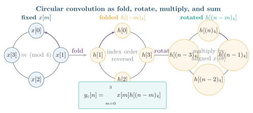
Four-point circular convolution. One sequence is fixed on a circle; the other is folded and rotated modulo four. Multiplying aligned samples and summing gives one output sample y_(c)(n).

Four-point circular convolution. One sequence is fixed on a circle; the other is folded and rotated modulo four. Multiplying aligned samples and summing gives one output sample $y_c(n)$ .

The graphical procedure mirrors linear convolution: hold $x[m]$ fixed, fold $h[m]$ to obtain $h[(-m)_N]$ , rotate it circularly by $n$ , multiply aligned samples, and sum. The essential difference is that all indices remain on an $N$ -point circle.

Direct, Tabular, and Matrix Methods

For hand calculation, construct the folded row

\bigl[h[0],h[N-1],h[N-2],\ldots,h[1]\bigr]

for $n=0$ , take its dot product with $[x[0],x[1],\ldots,x[N-1]]$ , and circularly shift the row one place to the right for each new output index. This is the tabular fold–rotate method in algebraic form.

Equivalently, let $\mathbf{x}=[x[0],\ldots,x[N-1]]^{\mathsf T}$ . Circular convolution is multiplication by a circulant matrix:

The entry in row $n$ , column $m$ is $h[(n-m)_N]$ . Every row is a one-place circular shift of the preceding row, which makes the modulo indexing visible and provides a reliable check on a hand-built table.

DFT Convolution Property

x[n]\longleftrightarrow X[k], \qquad h[n]\longleftrightarrow H[k],

are $N$ -point DFT pairs, then

Thus pointwise multiplication of two $N$ -point DFTs followed by an $N$ -point IDFT produces an $N$ -point circular convolution.

To prove the theorem, insert the circular-convolution sum into the DFT and put $r=(n-m)_N$ :

\begin{aligned} Y[k] &=\sum_{n=0}^{N-1}\sum_{m=0}^{N-1} x[m]h[(n-m)_N]W_N^{kn}\\ &=\sum_{m=0}^{N-1}x[m]W_N^{km} \sum_{r=0}^{N-1}h[r]W_N^{kr}\\ &=X[k]H[k]. \end{aligned}

The substitution is valid because, for fixed $m$ , modulo- $N$ addition merely permutes the $N$ values of $r$ . The dual property is

x[n]h[n]\longleftrightarrow \frac{1}{N}\bigl(X[k]\circledast_N H[k]\bigr).

Relationship to Linear Convolution

Let $y_\ell[n]=x[n]*h[n]$ be ordinary linear convolution and let $y_c[n]$ be their $N$ -point circular convolution after both inputs have been represented with length $N$ . Their exact wrap relation is

Shifted copies of the linear-convolution result overlap and add every $N$ samples. This wraparound is called time-domain aliasing.

Suppose the nonzero input lengths are $L$ and $M$ . The linear convolution has length at most $L+M-1$ . Choosing

N\geq L+M-1

prevents overlap because the complete result fits within one $N$ -sample period. Linear convolution can therefore be computed using a DFT as follows:

Choose a DFT length $N\geq L+M-1$ .
Zero-pad both sequences to length $N$ .
Compute the $N$ -point DFTs $X[k]$ and $H[k]$ .
Multiply bin by bin: $Y[k]=X[k]H[k]$ .
Take the $N$ -point IDFT of $Y[k]$ to obtain the linear convolution.

Without sufficient zero-padding, the IDFT instead returns aliased circular convolution.

Example — Why Zero-Padding Is Necessary

Let

x[0]=1,\quad x[1]=2, \qquad h[0]=1,\quad h[1]=1.

Without padding, their two-point circular convolution is

\begin{aligned} y_c[0] &=x[0]h[0]+x[1]h[1]=1+2=3,\\ y_c[1] &=x[0]h[1]+x[1]h[0]=1+2=3, \end{aligned}

and hence

\boxed{y_c[n]=\{3,3\}}.

The ordinary linear convolution is

\boxed{y_\ell[n]=\{1,3,2\}}.

For $N=2$ , the last linear-convolution sample wraps onto the first one exactly as predicted by the alias-sum formula:

y_c[0]=y_\ell[0]+y_\ell[2]=1+2=3.

Now use the required length $N=L+M-1=3$ and pad both inputs:

x=\{1,2,0\}, \qquad h=\{1,1,0\}.

Their three-point circular convolution is

\boxed{\{1,3,2\}=y_\ell[n]}.

The linear result now fits inside one period, so no samples overlap after wrapping. Zero-padding has converted the DFT’s inherent circular convolution into the required linear convolution.

Long-Sequence Fast Convolution

Transforming an indefinitely long input in one FFT is impractical. For an FIR impulse response of length $M$ , choose an FFT length $N\geq M$ and let

L=N-M+1

be the usual number of new input samples processed per block. Two standard block methods use $N$ -point circular convolutions while reproducing the exact linear convolution.

Overlap-Add Method

Divide the input into nonoverlapping blocks of $L$ samples.
Zero-pad each block and the $M$ -sample impulse response to length $N\geq L+M-1$ .
Compute an $N$ -point FFT, multiply by the precomputed $H[k]$ , and take the IFFT. Each block result is a length- $(L+M-1)$ linear convolution.
Place successive results $L$ samples apart and add their overlapping $M-1$ output samples.

Zeros prevent aliasing within each block; the final addition reconstructs the tails that neighbouring input blocks contribute to the same output samples.

Overlap-Save Method

Form each $N$ -sample input block from the previous $M-1$ samples and $L=N-M+1$ new samples. Adjacent input blocks overlap by $M-1$ .
Compute the $N$ -point circular convolution by FFT multiplication.
Discard the first $M-1$ output samples, which contain wraparound aliasing, and save the remaining $L$ valid samples.

Overlap-save uses no output addition and normally needs no input-block zero padding after the initial boundary block. Overlap-add pads blocks and adds output tails; overlap-save overlaps inputs and discards corrupted output heads. Both are exact when the stated lengths are respected.