Transmission of Signals and LTI Systems

Transmission of Signals

Signal transmission is the process of carrying information from a source to a destination through a physical medium such as copper cable, optical fibre, or free space.

A communication system converts the source information into a signal suited to the available channel and reconstructs the information at the destination. The transmitter may encode, pulse-shape, or modulate the message. The channel then introduces attenuation, bandwidth limitation, distortion, noise, and possibly interference. The receiver performs the complementary operations, such as channel selection, equalization, demodulation, decoding, and regeneration.

General communication chain: the transmitter conditions the source message for the physical channel, noise and other impairments alter the received signal, and the receiver reconstructs the message for the destination.

Baseband and Passband Transmission

Baseband Transmission

In baseband transmission, the information-bearing waveform is sent directly without translation to a high-frequency carrier. Its spectrum remains centred about zero frequency (DC). For digital data, the bit sequence is converted to a line-coded pulse waveform, such as NRZ or Manchester code, and applied directly to a low-pass channel.

Baseband transmission is appropriate when the medium passes frequencies down to or near DC. The transmitter mainly performs line coding and pulse shaping; the receiver uses filtering, equalization, timing recovery, pulse detection, and regeneration. It is simple and efficient on dedicated wired links, but it cannot directly share a radio-frequency channel by carrier allocation.

• Digital data over short wired links

• Ethernet baseband signalling

• PCM pulses before modulation

Passband Transmission

In passband transmission, the message modifies a parameter of a sinusoidal carrier and shifts its spectrum from baseband to a band centred about the carrier frequency $f_c$. A general modulated waveform can be written as

Caution

Key Formula — General passband signal

$$s(t)=A(t)\cos\!\left[\omega_ct+\phi(t)\right],$$

where the message controls the amplitude $A(t)$, phase $\phi(t)$, or instantaneous frequency. For example, multiplication by a carrier gives $s(t)=m(t)\cos\omega_ct$ and creates translated spectral components around $\pm\omega_c$.

Modulation permits practical antenna dimensions, efficient radiation, frequency-division multiplexing, spectrum allocation, and transmission through band-pass media. The transmitter therefore contains a modulator and RF stages, while the receiver selects the wanted channel and demodulates it back to baseband.

• AM, FM, and PM radio

• Mobile communication

• Satellite communication

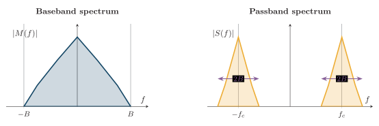
A baseband spectrum is centred at zero frequency; multiplication by a carrier translates copies of the spectrum to bands centred at $\pm f_c$.

Feature	Baseband transmission	Passband transmission
Spectral location	Centred near $0$ Hz	Centred near carrier $f_c$
Carrier modulation	Not required	Required
Typical medium	Wired low-pass channel	Radio, satellite, or band-pass cable channel
Main transmitter operation	Line coding and pulse shaping	Modulation and frequency translation
Receiver operation	Equalization and pulse detection	RF selection, demodulation, then baseband recovery

Comparison of baseband and passband transmission.

Factors Affecting Transmission

Factor	Effect
Bandwidth limitation	Causes waveform spreading and intersymbol interference
Noise	Adds a random disturbance and reduces $S/N$
Attenuation	Decreases signal power with distance
Distortion	Alters different frequency components unequally
Interference	Adds unwanted signals from other sources

Principal transmission impairments.

Distortionless Transmission

Note

Law — Distortionless-transmission condition

A system is distortionless for an input $x(t)$ if its output is only a scaled and delayed replica,

$$y(t)=Kx(t-t_d).$$

Equivalently, over the occupied frequency band of the input,

$$H(\omega)=K\,e^{-\mathrm{j}\omega t_d},\qquad \lvert H(\omega)\rvert=K,\qquad \angle H(\omega)=-\omega t_d.$$

The constant magnitude prevents amplitude distortion. The phase is linear in $\omega$, so every occupied spectral component has the same delay $t_d$ and there is no phase distortion. These conditions are required only over the input signal’s occupied band, not necessarily at every frequency.

Tip

Exam Focus

For a distortionless-channel question, state all three ideas: scaled and delayed output, constant magnitude response, and linear phase over the signal band. Do not repeat the bandwidth–SNR capacity calculation from the previous section; it concerns channel rate rather than waveform fidelity.

Linear Time-Invariant Systems

An LTI system is a system that satisfies both linearity and time invariance. Its behaviour is completely described by its impulse response.

Linearity

Let $\mathcal{T}$ denote a system. It is linear if it obeys superposition:

Note

Law — Linearity test

If $x_1\xrightarrow{\mathcal{T}}y_1$ and $x_2\xrightarrow{\mathcal{T}}y_2$, then for arbitrary constants $a$ and $b$,

$$ax_1+bx_2\xrightarrow{\mathcal{T}}ay_1+by_2,$$

or equivalently

$$\mathcal{T}\{ax_1+bx_2\} =a\mathcal{T}\{x_1\}+b\mathcal{T}\{x_2\}.$$

The two parts of superposition are additivity, obtained by taking $a=b=1$, and homogeneity, obtained by considering one scaled input.

Time Invariance

A system is time invariant when delaying the input merely delays the output by the same amount; the system itself does not depend on absolute time.

Note

Law — Time-invariance test

For continuous time,

$$x(t)\longrightarrow y(t) \quad\Rightarrow\quad x(t-t_0)\longrightarrow y(t-t_0).$$

For discrete time,

$$x[n]\longrightarrow y[n] \quad\Rightarrow\quad x[n-n_0]\longrightarrow y[n-n_0].$$

When both tests hold, the input-output relation is convolution with the system’s impulse response:

Caution

Key Formula — LTI input-output relations

$$y(t)=x(t)*h(t), \qquad y[n]=x[n]*h[n].$$

Two especially important LTI properties can already be read from $h$.

Property	Continuous-time condition	Discrete-time condition
Causal	$h(t)=0$ for $t<0$	$h[n]=0$ for $n<0$
BIBO stable	$\displaystyle\int_{-\infty}^{\infty}\lvert h(t)\rvert\,\mathrm{d}t<\infty$	$\displaystyle\sum_{n=-\infty}^{\infty}\lvert h[n]\rvert<\infty$

Causality and BIBO-stability tests for LTI systems.

BIBO stability means that every bounded input produces a bounded output. The impulse-response derivations below justify both conditions.

Impulse Response

The impulse response is the output of a system when its input is a unit impulse. Thus

$$x(t)=\delta(t)\Rightarrow y(t)=h(t), \qquad x[n]=\delta[n]\Rightarrow y[n]=h[n].$$

Applying a unit impulse to an LTI system produces its impulse response, which completely characterizes the system.

For an LTI system, $h(t)$ or $h[n]$ completely characterizes the system: once it is known, convolution gives the output for every admissible input.

Why the Impulse Is the Natural Test Signal

Every signal can be synthesized from scaled and shifted impulses. The sifting property gives the discrete decomposition

$$x[n]=\sum_{k=-\infty}^{\infty}x[k]\,\delta[n-k]$$

and the continuous decomposition

$$x(t)=\int_{-\infty}^{\infty} x(\tau)\,\delta(t-\tau)\,\mathrm{d}\tau.$$

Time invariance makes the response to a shifted impulse $\delta[n-k]$ equal to the shifted impulse response $h[n-k]$. Linearity then permits each response to be weighted by $x[k]$ and all responses to be added. Therefore

$$y[n]=\sum_{k=-\infty}^{\infty}x[k]h[n-k]=x[n]*h[n].$$

The same argument in continuous time yields

$$y(t)=\int_{-\infty}^{\infty}x(\tau)h(t-\tau)\,\mathrm{d}\tau=x(t)*h(t).$$

Thus the impulse response is a complete “fingerprint” of an LTI system: it records the response to the elementary components from which every input is formed.

System Properties from the Impulse Response

Property	Continuous-time condition	Discrete-time condition	Meaning
Memoryless	$h(t)=K\delta(t)$	$h[n]=K\delta[n]$	Output depends only on the present input
Causal	$h(t)=0$ for $t<0$	$h[n]=0$ for $n<0$	No output before the input is applied
BIBO stable	$\displaystyle\int_{-\infty}^{\infty}\lvert h(t)\rvert\,\mathrm{d}t<\infty$	$\displaystyle\sum_{n=-\infty}^{\infty}\lvert h[n]\rvert<\infty$	Every bounded input gives a bounded output
Invertible	$\exists h_{\mathrm{inv}}:\ h*h_{\mathrm{inv}}=\delta(t)$	$\exists h_{\mathrm{inv}}:\ h*h_{\mathrm{inv}}=\delta[n]$	The input can be recovered from the output

Complete impulse-response tests for common LTI-system properties.

These conditions follow directly from convolution.

• Memoryless: If $h(t)=K\delta(t)$, then $y(t)=x(t)*K\delta(t)=Kx(t)$, so the output uses only the present input. Any delayed or spread component of $h(t)$ introduces memory.

• Causal: In $y(t)=\int x(\tau)h(t-\tau)\,\mathrm{d}\tau$, causality forbids dependence on future values $\tau>t$. This is guaranteed precisely when $h(t-\tau)=0$ for $t-\tau<0$, or $h(v)=0$ for $v<0$.

• Stable: If $\lvert x(t)\rvert\leq M$, the convolution bound gives

$$\begin{aligned} \lvert y(t)\rvert &\leq\int_{-\infty}^{\infty} \lvert x(\tau)\rvert\lvert h(t-\tau)\rvert\,\mathrm{d}\tau\\ &\leq M\int_{-\infty}^{\infty}\lvert h(v)\rvert\,\mathrm{d}v. \end{aligned}$$

Absolute integrability of $h(t)$ therefore guarantees a bounded output. The discrete proof replaces the integral by a sum.

• Invertible: Cascading a system with its inverse must produce the identity system, whose impulse response is $\delta$. Hence $h*h_{\mathrm{inv}}=\delta$.

Note

Key Point — BIBO criterion

For an LTI system, BIBO stability holds if and only if its impulse response is absolutely integrable in continuous time or absolutely summable in discrete time. This is one of the most frequently examined impulse-response tests.

[!NOTE]

Example — Causality and Stability from the Impulse Response

Determine whether

$$h(t)=e^{-2t}u(t)$$

is causal and BIBO stable.

Because $u(t)=0$ for $t<0$, the impulse response is zero for negative time and the system is causal. Moreover,

$$\int_{-\infty}^{\infty}\lvert h(t)\rvert\,\mathrm{d}t =\int_0^\infty e^{-2t}\,\mathrm{d}t =\frac12<\infty.$$

Hence the system is also BIBO stable.

For contrast, $h(t)=u(t)$ is causal but unstable because its absolute integral is infinite. The response $h(t)=e^tu(-t)$ is stable because $\int_{-\infty}^{0}e^t\,\mathrm{d}t=1$, but it is noncausal because it is nonzero for $t<0$.

Step Response and Impulse Response

The step response $s(t)$ is the output produced by the unit-step input $u(t)$. Because the unit step is the running integral of the impulse, the step and impulse responses form an integral–derivative pair:

Caution

Key Formula — Continuous-time response pair

$$s(t)=\int_{-\infty}^{t}h(\tau)\,\mathrm{d}\tau, \qquad h(t)=\frac{\mathrm{d}s(t)}{\mathrm{d}t}.$$

For discrete time, accumulation and first difference give

Caution

Key Formula — Discrete-time response pair

$$s[n]=\sum_{k=-\infty}^{n}h[k], \qquad h[n]=s[n]-s[n-1].$$

Either response can therefore be obtained from the other, a common short-question variation.

Transfer Function and Eigenfunctions

Transforming the impulse response gives the system transfer function or frequency response:

Caution

Key Formula — Transforms of the impulse response

$$H(s)=\int_{-\infty}^{\infty}h(t)e^{-st}\,\mathrm{d}t, \qquad H(\omega)=\int_{-\infty}^{\infty}h(t)e^{-\mathrm{j}\omega t}\,\mathrm{d}t.$$

Thus $H(s)=\mathcal{L}\{h(t)\}$ and $H(\omega)=\mathcal{F}\{h(t)\}$. Convolution in time becomes multiplication in either transform domain:

$$y=x*h \quad\Longleftrightarrow\quad Y(s)=X(s)H(s), \qquad Y(\omega)=X(\omega)H(\omega).$$

Complex exponentials are eigenfunctions of every LTI system. For $x(t)=e^{st}$,

$$\begin{aligned} y(t) &=\int_{-\infty}^{\infty}h(\tau)e^{s(t-\tau)}\,\mathrm{d}\tau\\ &=e^{st}\int_{-\infty}^{\infty}h(\tau)e^{-s\tau}\,\mathrm{d}\tau\\ &=H(s)e^{st}. \end{aligned}$$

The waveform is unchanged; the system only scales it by the eigenvalue $H(s)$.

Finally, impulse-response duration classifies digital filters.

Impulse response	Filter type
Finite duration (finitely many nonzero terms)	FIR
Infinite duration	IIR

Digital-filter classification by impulse-response duration.

These filter classes are developed in detail later in this chapter.

Convolution

Convolution combines an input signal with the impulse response of an LTI system to determine its output. It accounts for the response produced by every input value and adds all contributions at the observation time.

For continuous-time signals,

Caution

Key Formula — Continuous-time convolution

$$y(t)=x(t)*h(t) =\int_{-\infty}^{\infty}x(\tau)h(t-\tau)\,\mathrm{d}\tau.$$

For discrete-time signals,

Caution

Key Formula — Discrete-time convolution

$$y[n]=x[n]*h[n] =\sum_{k=-\infty}^{\infty}x[k]h[n-k].$$

Derivation from the LTI Properties

Any continuous-time input can be decomposed into a continuum of shifted impulses:

$$x(t)=\int_{-\infty}^{\infty} x(\tau)\delta(t-\tau)\,\mathrm{d}\tau.$$

The term $x(\tau)\delta(t-\tau)\,\mathrm{d}\tau$ represents an impulse at $t=\tau$ with infinitesimal weight $x(\tau)\,\mathrm{d}\tau$. If the response to $\delta(t)$ is $h(t)$, time invariance makes the response to $\delta(t-\tau)$ equal to $h(t-\tau)$. By linearity, that response is weighted by $x(\tau)\,\mathrm{d}\tau$, and all such responses can be superposed. Consequently,

$$\boxed{y(t)=\int_{-\infty}^{\infty} x(\tau)h(t-\tau)\,\mathrm{d}\tau=x(t)*h(t)}.$$

Similarly, the discrete decomposition

$$x[n]=\sum_{k=-\infty}^{\infty}x[k]\delta[n-k]$$

gives

$$\boxed{y[n]=\sum_{k=-\infty}^{\infty} x[k]h[n-k]=x[n]*h[n]}.$$

Convolution is therefore not merely a calculation rule; it follows directly from linearity and time invariance.

Graphical Convolution Procedure

For graphical continuous-time convolution, keep $x(\tau)$ fixed and operate on $h(\tau)$:

1. Fold: Reflect $h(\tau)$ about the vertical axis to obtain $h(-\tau)$.

2. Shift: Move the folded signal by the observation time $t$ to obtain $h(t-\tau)$.

3. Multiply: Form the point-by-point product $x(\tau)h(t-\tau)$.

4. Integrate: The signed area of that product is the single output value $y(t)$.

5. Slide and repeat: Vary $t$ from $-\infty$ to $+\infty$ to construct the complete output waveform.

The output is large when the two waveforms have substantial overlap and is zero when they do not overlap.

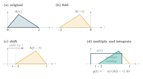
Graphical convolution: fold $h(\tau)$, shift it to $h(t-\tau)$, multiply by the fixed $x(\tau)$, and integrate the signed overlap area to obtain one value of $y(t)$.

Properties of Convolution

The following properties hold whenever the stated convolutions, integrals, or sums exist. They simplify interconnected LTI systems and are frequently asked directly in examinations.

Commutative property.

Note

Law — Commutativity

$$x(t)*h(t)=h(t)*x(t).$$

Starting with the definition and substituting $\lambda=t-\tau$,

$$\begin{aligned} \int_{-\infty}^{\infty}x(\tau)h(t-\tau)\,\mathrm{d}\tau &=\int_{-\infty}^{\infty}h(\lambda)x(t-\lambda)\,\mathrm{d}\lambda, \end{aligned}$$

which is $h*x$. Therefore the order of the two signals does not affect the result.

Associative property.

Note

Law — Associativity

$$x*(h*g)=(x*h)*g.$$

The grouping of successive convolutions can be changed without changing the output. Physically, two LTI systems with impulse responses $h$ and $g$ in cascade have the overall impulse response $h*g$, regardless of which pair is convolved first. A complicated cascade may therefore be replaced by one equivalent system.

Distributive property.

Note

Law — Distributivity

$$x*(h+g)=x*h+x*g.$$

Distribution of the convolution integral over addition gives

$$\begin{aligned} &\int_{-\infty}^{\infty} x(\tau)\bigl[h(t-\tau)+g(t-\tau)\bigr] \,\mathrm{d}\tau\\ &\qquad=\int_{-\infty}^{\infty}x(\tau)h(t-\tau)\,\mathrm{d}\tau +\int_{-\infty}^{\infty}x(\tau)g(t-\tau)\,\mathrm{d}\tau. \end{aligned}$$

This represents parallel LTI systems: their total output is the sum of the individual outputs.

Identity and impulse-shift property.

The unit impulse is the identity element of convolution:

$$\boxed{x(t)*\delta(t)=x(t)}.$$

The sifting property also gives

$$\begin{aligned} x(t)*\delta(t-t_0) &=\int_{-\infty}^{\infty} x(\tau)\delta(t-t_0-\tau)\,\mathrm{d}\tau\\ &=\boxed{x(t-t_0)}. \end{aligned}$$

Convolution with an impulse reproduces the signal; a shifted impulse reproduces and shifts it.

Time-shift property.

If $y(t)=x(t)*h(t)$, delaying either signal delays the output by the same amount, while delaying both adds the delays:

Caution

Key Formula — Convolution time shift

$$x(t-t_1)*h(t-t_2)=y(t-t_1-t_2).$$

The single-shift case $x(t-t_0)*h(t)=x(t)*h(t-t_0)=y(t-t_0)$ is the convolution form of time invariance.

Time-scaling property.

Compressing or expanding the time axes of both signals by the same nonzero factor $a$ scales the output in time and its amplitude by $1/\lvert a\rvert$:

Caution

Key Formula — Convolution time scaling

$$x(at)*h(at)=\frac{1}{\lvert a\rvert}y(at), \qquad a\neq0.$$

Differentiation property.

When the derivatives exist and differentiation can be interchanged with the convolution integral,

Caution

Key Formula — Differentiation of a convolution

$$\frac{\mathrm{d}}{\mathrm{d}t}(x*h) =\frac{\mathrm{d}x}{\mathrm{d}t}*h =x*\frac{\mathrm{d}h}{\mathrm{d}t}.$$

This is useful for differential-equation problems and for moving between step and impulse responses.

Area and duration properties.

For absolutely integrable signals, the area under a convolution is the product of the individual areas:

Caution

Key Formula — Area of a convolution

$$\int_{-\infty}^{\infty}(x*h)(t)\,\mathrm{d}t =\left(\int_{-\infty}^{\infty}x(t)\,\mathrm{d}t\right) \left(\int_{-\infty}^{\infty}h(t)\,\mathrm{d}t\right).$$

If finite-duration signals occupy intervals of lengths $T_x$ and $T_h$, their convolution generally has duration $T_x+T_h$, apart from endpoint conventions or cancellation. It starts at first overlap and ends when the overlap disappears. For finite discrete sequences of lengths $L_x$ and $L_h$, the linear-convolution length is $L_x+L_h-1$.

Convolution theorem.

Convolution in time is pointwise multiplication in frequency:

Note

Law — Convolution theorem

$$\mathcal{F}\{x(t)*h(t)\}=X(\omega)H(\omega).$$

The corresponding Laplace-domain relation is

$$\mathcal{L}\{x(t)*h(t)\}=X(s)H(s).$$

The transform turns a difficult convolution integral into an algebraic product. This is the basis of transfer-function analysis, where the output transform equals the input transform multiplied by the system transfer function.

Discrete Convolution Example

Note

Example — Convolution of Two Length-Two Sequences

Let $x[0]=1$, $x[1]=2$, $h[0]=1$, and $h[1]=1$, with all other samples zero. Find $y[n]=x[n]*h[n]$.

The result has length $2+2-1=3$. From

$$y[n]=\sum_{k=-\infty}^{\infty}x[k]h[n-k],$$

the nonzero samples are

$$\begin{aligned} y[0]&=1\times1=1,\\ y[1]&=1\times1+2\times1=3,\\ y[2]&=2\times1=2. \end{aligned}$$

Therefore

$$\boxed{y[0]=1,\qquad y[1]=3,\qquad y[2]=2}.$$

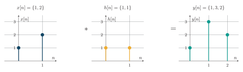
Discrete linear convolution of $x(n)=\{1,2\}$ and $h(n)=\{1,1\}$ produces the three-sample sequence $y(n)=\{1,3,2\}$.

Rectangular-Pulse Convolution

Let $x(t)=h(t)=1$ for $0\leq t\leq1$ and let both signals be zero elsewhere. At each shift, the convolution integral equals the overlap length of the two unit-width pulses. Hence

Caution

Key Formula — Unit rectangular pulses

$$y(t)= \begin{cases} 0, & t<0,\\ t, & 0\leq t\leq1,\\ 2-t, & 1<t\leq2,\\ 0, & t>2. \end{cases}$$

The output is triangular and is supported on $0\leq t\leq2$. More generally, convolving finite-duration signals of widths $T_x$ and $T_h$ produces support of width $T_x+T_h$ between first and last overlap, subject to endpoint conventions and possible cancellation.

Quick Review

Note

Key Point — Exam-ready facts

• Baseband transmission uses no carrier and a low-pass channel; passband transmission modulates the message onto a carrier.

• Distortionless transmission requires $y(t)=Kx(t-t_d)$, constant $\lvert H(\omega)\rvert$, and linear phase over the occupied signal band.

• LTI means linearity plus time invariance, and an LTI system is fully described by its impulse response $h$.

• The LTI output is the convolution of the input and impulse response: $y=x*h$.

• Causality requires $h(t)=0$ for $t<0$; BIBO stability requires $h$ to be absolutely integrable or absolutely summable.

• Graphical convolution uses fold $\rightarrow$ shift $\rightarrow$ multiply $\rightarrow$ integrate; convolution is commutative, associative, and distributive.

• Convolution in time corresponds to multiplication $X(\omega)H(\omega)$ in frequency.