Fourier Series and Fourier Transform

Fourier analysis resolves a signal into complex exponentials, which are eigenfunctions of every linear time-invariant (LTI) system. A continuous-time periodic signal requires a discrete set of harmonically related exponentials and is described by a Fourier series. A typical aperiodic energy signal requires a continuum of frequencies and is described by a Fourier transform. Throughout this chapter,

$$\omega=2\pi f.$$

Here $f$ is cyclic frequency in hertz and $\omega$ is angular frequency in radians per second. Keeping this convention fixed determines every factor of $2\pi$.

Fourier Series of a Periodic Signal

Let $x(t+T_0)=x(t)$, where $T_0$ is the fundamental period, and let $\omega_0=2\pi/T_0$. The frequencies $n\omega_0$, $n\in\mathbb Z$, are the DC component, fundamental, and harmonics.

Complex Exponential Form

$$\begin{aligned} x(t)&=\sum_{n=-\infty}^{\infty}C_ne^{\mathrm{j}n\omega_0t},\\ C_n&=\frac{1}{T_0}\int_{t_0}^{t_0+T_0} x(t)e^{-\mathrm{j}n\omega_0t}\,\mathrm{d}t. \end{aligned}$$

The coefficient integral may be evaluated over any complete period; its value is independent of the starting point $t_0$.

For integers $m$ and $n$, the complex harmonics obey

Caution

Key Formula — Orthogonality of complex harmonics

$$\frac{1}{T_0}\int_{t_0}^{t_0+T_0} e^{\mathrm{j}n\omega_0t}e^{-\mathrm{j}m\omega_0t}\,\mathrm{d}t =\delta_{nm} = \begin{cases} 1, & n=m,\\ 0, & n\neq m. \end{cases}$$

Here $\delta_{nm}$ is the Kronecker delta, not the Dirac impulse. Multiplying the series by $e^{-\mathrm{j}m\omega_0t}$ and integrating over one period isolates $C_m$. In particular,

$$C_0=\frac{1}{T_0}\int_{t_0}^{t_0+T_0}x(t)\,\mathrm{d}t$$

is the average or DC value.

Trigonometric Form

For a real periodic signal, an equivalent representation is

Caution

Key Formula — Trigonometric Fourier series

$$\begin{aligned} x(t)&=a_0+\sum_{n=1}^{\infty} \left[a_n\cos(n\omega_0t)+b_n\sin(n\omega_0t)\right],\\ a_0&=\frac{1}{T_0}\int_{t_0}^{t_0+T_0}x(t)\,\mathrm{d}t,\\ a_n&=\frac{2}{T_0}\int_{t_0}^{t_0+T_0} x(t)\cos(n\omega_0t)\,\mathrm{d}t,\qquad n\geq1,\\ b_n&=\frac{2}{T_0}\int_{t_0}^{t_0+T_0} x(t)\sin(n\omega_0t)\,\mathrm{d}t,\qquad n\geq1. \end{aligned}$$

Sine and cosine orthogonality gives these coefficients in the same way. This section uses $a_0$ itself as the average. The alternative convention with $a_0/2$ as the constant term assigns a different meaning to the symbol $a_0$; the two conventions must not be mixed.

Euler’s identities give the exact conversion between forms.

Quantity	Conversion
DC term	$C_0=a_0$
Positive-frequency coefficient	$\displaystyle C_n=\frac{a_n-\mathrm{j}b_n}{2}$, $n\geq1$
Negative-frequency coefficient	$\displaystyle C_{-n}=\frac{a_n+\mathrm{j}b_n}{2}$, $n\geq1$
Cosine coefficient	$a_n=C_n+C_{-n}$
Sine coefficient	$b_n=\mathrm{j}(C_n-C_{-n})$

Conversion between complex and trigonometric Fourier coefficients.

For real $x(t)$, $C_{-n}=C_n^*$. Pairing positive and negative frequencies gives

Caution

Key Formula — One-sided harmonic amplitude and phase

$$x(t)=C_0+\sum_{n=1}^{\infty}A_n\cos(n\omega_0t+\phi_n), \qquad A_n=2|C_n|=\sqrt{a_n^2+b_n^2}, \qquad \phi_n=\arg C_n.$$

Equivalently, $a_n=A_n\cos\phi_n$ and $b_n=-A_n\sin\phi_n$. A two-sided complex spectrum uses line height $|C_n|$ at each signed frequency, while a one-sided sinusoidal amplitude spectrum uses $2|C_n|$ for $n>0$.

Frequency and Line-Spectrum Interpretation

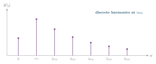
The coefficient $C_n$ specifies the complex amplitude of the spectral line at $\omega=n\omega_0$. No content exists between adjacent harmonics.

Fourier-series line spectrum with discrete amplitudes at harmonic multiples of the fundamental angular frequency.

Since

$$\mathcal{F}\!\left\{e^{\mathrm{j}n\omega_0t}\right\}=2\pi\delta(\omega-n\omega_0),$$

the generalized transform of the periodic signal is

Caution

Key Formula — Transform of a continuous-time periodic signal

$$x(t)=\sum_{n=-\infty}^{\infty}C_ne^{\mathrm{j}n\omega_0t} \quad\Longleftrightarrow\quad X(\omega)=2\pi\sum_{n=-\infty}^{\infty} C_n\delta(\omega-n\omega_0).$$

A nonzero periodic signal generally is not absolutely integrable over the whole real line, so this impulse train is a distributional transform rather than an ordinary convergent Fourier integral.

Feature	Periodic signal	Typical aperiodic energy signal
Representation	Fourier-series coefficients $C_n$	Fourier transform $X(\omega)$
Frequency variable	Discrete harmonics $n\omega_0$	Continuous angular frequency $\omega$
Generalized FT	Weighted impulse lines	Usually an ordinary continuous spectrum
Natural measure	Average power	Total energy
Parseval form	Sum over $n$	Integral over $\omega$

Continuous-time periodic and aperiodic Fourier descriptions.

Aperiodicity alone does not guarantee finite energy or an ordinary transform; general signals can also contain mixtures of continuous spectra and lines.

Symmetry Shortcuts

Before integrating, inspect the waveform over a symmetric period. The following rules often remove most of the calculation.

Signal condition	Trigonometric result	Complex-coefficient result
Real, $x(t)\in\mathbb R$	$a_n,b_n\in\mathbb R$	$C_{-n}=C_n^*$
Even, $x(-t)=x(t)$	$b_n=0$; cosine terms only	$C_{-n}=C_n\in\mathbb R$
Odd, $x(-t)=-x(t)$	$a_0=a_n=0$; sine terms only	$C_{-n}=-C_n$ and $C_n$ is imaginary
Half-wave, $x(t+T_0/2)=-x(t)$	No DC or even harmonics	$C_n=0$ for every even $n$

Fourier-series symmetry rules for a real periodic signal.

For half-wave symmetry, splitting the coefficient integral into two half periods produces the factor $1-(-1)^n$, which vanishes for even $n$. Half-wave symmetry alone does not eliminate all sine terms or all cosine terms; even or odd symmetry is needed for that additional simplification.

Convergence and the Gibbs Phenomenon

Note

Law — Dirichlet convergence conditions

A standard sufficient set of conditions over one period is that $x(t)$ is absolutely integrable, has only finitely many maxima and minima, and has only finitely many finite jump discontinuities. Piecewise continuously differentiable signals satisfy these conditions. They are sufficient, not necessary.

If $S_N(t)=\sum_{n=-N}^{N}C_ne^{\mathrm{j}n\omega_0t}$, then

$$\lim_{N\to\infty}S_N(t) =\frac{x(t^-)+x(t^+)}{2}.$$

Hence the series converges to $x(t)$ at a continuity point and to the midpoint of the one-sided limits at a jump.

Near a jump of height $\Delta=|x(t^+)-x(t^-)|$, a truncated series oscillates. As the number of harmonics grows, the limiting maximum overshoot above the upper one-sided level is approximately

$$0.08949\,\Delta\approx9\%\text{ of the jump height}.$$

There is a corresponding undershoot on the other side. This fractional peak does not tend to zero; only the width of the oscillatory region shrinks toward the discontinuity. Away from the jump the approximation improves, and at the jump itself it converges to the midpoint. This is the Gibbs phenomenon.

Note

Example — Fourier Series of a Symmetric Square Wave

Let the $T_0$-periodic waveform be

$$x(t)= \begin{cases} -A, & -T_0/2<t<0,\\ A, & 0<t<T_0/2, \end{cases} \qquad A>0.$$

It is odd and has half-wave symmetry. Therefore $a_0=a_n=0$, and only odd sine harmonics can remain. Direct calculation gives

$$\begin{aligned} b_n &=\frac{2}{T_0}\int_{-T_0/2}^{T_0/2} x(t)\sin(n\omega_0t)\,\mathrm{d}t\\ &=\frac{4A}{T_0}\int_0^{T_0/2}\sin(n\omega_0t)\,\mathrm{d}t\\ &=\frac{2A}{n\pi}\left[1-(-1)^n\right] = \begin{cases} \dfrac{4A}{n\pi}, & n\text{ odd},\\[4pt] 0, & n\text{ even}. \end{cases} \end{aligned}$$

Thus

$$\boxed{x(t)=\frac{4A}{\pi} \left[\sin\omega_0t+\frac{1}{3}\sin3\omega_0t +\frac{1}{5}\sin5\omega_0t+\cdots\right]}.$$

For nonzero odd $n$, the complex coefficients are

$$C_n=-\mathrm{j}\frac{2A}{n\pi}, \qquad C_n=0\text{ for even }n, \qquad C_0=0.$$

At every switching instant, the series converges to the midpoint $0$, not to an arbitrarily assigned endpoint value. Partial sums exhibit the persistent Gibbs overshoot there.

Parseval Relation for a Fourier Series

Orthogonality divides average power among the harmonic lines:

Caution

Key Formula — Fourier-series Parseval relation

$$P_x=\frac{1}{T_0}\int_{t_0}^{t_0+T_0}|x(t)|^2\,\mathrm{d}t =\sum_{n=-\infty}^{\infty}|C_n|^2.$$

For a real signal in this section’s trigonometric convention,

$$P_x=a_0^2+\frac{1}{2}\sum_{n=1}^{\infty}(a_n^2+b_n^2).$$

For the square wave, $P_x=A^2$. Substitution of its sine coefficients gives

$$A^2=\frac{8A^2}{\pi^2} \sum_{k=0}^{\infty}\frac{1}{(2k+1)^2},$$

consistent with $\sum_{k=0}^{\infty}(2k+1)^{-2}=\pi^2/8$.

Continuous-Time Fourier Transform

$$\begin{aligned} X(\omega)&=\mathcal{F}\!\left\{x(t)\right\} =\int_{-\infty}^{\infty}x(t)e^{-\mathrm{j}\omega t}\,\mathrm{d}t,\\ x(t)&=\mathcal{F}^{-1}\!\left\{X(\omega)\right\} =\frac{1}{2\pi}\int_{-\infty}^{\infty} X(\omega)e^{\mathrm{j}\omega t}\,\mathrm{d}\omega. \end{aligned}$$

We write the transform pair as $x(t)\longleftrightarrow X(\omega)$.

Absolute integrability,

$$\int_{-\infty}^{\infty}|x(t)|\,\mathrm{d}t<\infty,$$

is a useful sufficient condition for the ordinary transform to exist; it is not necessary. Finite-energy signals admit an $L^2$ transform in the mean-square sense, while constants, sinusoids, and impulses are handled by generalized functions or distributions. Under the $L^1$ condition, $X(\omega)$ is bounded and continuous and tends to zero as $|\omega|\to\infty$.

Physical Meaning of Magnitude and Phase

The waveform $x(t)$ describes variation with time, while

$$X(\omega)=|X(\omega)|e^{\mathrm{j}\angle X(\omega)}$$

describes the magnitude density and phase of its frequency components. The inverse transform shows that a narrow interval $\mathrm{d}\omega$ contributes approximately

$$\frac{1}{2\pi}X(\omega)e^{\mathrm{j}\omega t}\,\mathrm{d}\omega$$

to the signal. Therefore $X(\omega)$ is a spectral density, not generally the amplitude of one isolated sinusoid. If $x$ has units $U$, then $X$ has units $U\cdot\mathrm{s}$ under this convention.

The magnitude $|X(\omega)|$ measures frequency content, while $\angle X(\omega)$ determines how components align in time. Magnitude alone usually cannot reconstruct the waveform. Phase is undefined at spectral zeros and is interpreted modulo $2\pi$ when wrapped.

Real-Signal Symmetry

For a real signal, the spectrum is Hermitian:

Caution

Key Formula — Hermitian symmetry

$$X(-\omega)=X^*(\omega).$$

Hence $|X(\omega)|$ is even and phase is odd wherever a consistent phase branch is defined.

Time-domain condition	Frequency-domain consequence
$x(t)$ real	$X(-\omega)=X^*(\omega)$
$x(t)$ real and even	$X(\omega)$ is real and even
$x(t)$ real and odd	$X(\omega)$ is imaginary and odd
$x^*(t)$	$X^*(-\omega)$
$x(-t)$	$X(-\omega)$

Useful Fourier-transform symmetry results.

Fourier-Transform Properties

Assume $x(t)\longleftrightarrow X(\omega)$ and $g(t)\longleftrightarrow G(\omega)$. Frequency-domain convolution means

$$(X*G)(\omega)=\int_{-\infty}^{\infty} X(\nu)G(\omega-\nu)\,\mathrm{d}\nu.$$

Property	Time-domain expression	Frequency-domain expression
Linearity	$a x(t)+b g(t)$	$aX(\omega)+bG(\omega)$
Time shift	$x(t-t_0)$	$e^{-\mathrm{j}\omega t_0}X(\omega)$
Frequency shift	$e^{\mathrm{j}\omega_0t}x(t)$	$X(\omega-\omega_0)$
Time scaling, $a\neq0$	$x(at)$	$\dfrac{1}{
Time differentiation	$\dfrac{\mathrm{d}x(t)}{\mathrm{d}t}$	$\mathrm{j}\omega X(\omega)$
Convolution	$x(t)*g(t)$	$X(\omega)G(\omega)$
Multiplication	$x(t)g(t)$	$\dfrac{1}{2\pi}(X*G)(\omega)$
Duality	$X(t)$	$2\pi x(-\omega)$
Real-signal symmetry	$x(t)\in\mathbb R$	$X(-\omega)=X^*(\omega)$
Parseval energy	$\displaystyle\int_{-\infty}^{\infty}	x(t)

Properties for the angular-frequency Fourier convention.

The derivations below assume the required integrals, changes of integration order, derivatives, and boundary terms are valid. The identities also hold distributionally when interpreted appropriately.

Concise Derivations

Linearity.

Linearity of integration gives

$$\mathcal{F}\!\left\{a x(t)+b g(t)\right\} =\int_{-\infty}^{\infty}[a x(t)+b g(t)]e^{-\mathrm{j}\omega t}\,\mathrm{d}t =aX(\omega)+bG(\omega).$$

Time shifting.

With $\tau=t-t_0$,

$$\begin{aligned} \mathcal{F}\!\left\{x(t-t_0)\right\} &=\int_{-\infty}^{\infty}x(\tau) e^{-\mathrm{j}\omega(\tau+t_0)}\,\mathrm{d}\tau\\ &=e^{-\mathrm{j}\omega t_0}X(\omega). \end{aligned}$$

A delay changes phase by $-\omega t_0$ but leaves magnitude unchanged.

Frequency shifting.

Combining the exponentials yields

$$\mathcal{F}\!\left\{e^{\mathrm{j}\omega_0t}x(t)\right\} =\int_{-\infty}^{\infty}x(t) e^{-\mathrm{j}(\omega-\omega_0)t}\,\mathrm{d}t =X(\omega-\omega_0).$$

Multiplication by a complex carrier translates the spectrum by $+\omega_0$, which is the mathematical basis of modulation.

Time scaling.

For $\tau=at$, reversing the limits when $a<0$ gives

$$\mathcal{F}\!\left\{x(at)\right\}=\frac{1}{|a|} \int_{-\infty}^{\infty}x(\tau) e^{-\mathrm{j}(\omega/a)\tau}\,\mathrm{d}\tau =\frac{1}{|a|}X\!\left(\frac{\omega}{a}\right).$$

Compression in time expands the spectrum, and expansion in time compresses it.

Differentiation in time.

Integration by parts gives

$$\begin{aligned} \mathcal{F}\!\left\{\frac{\mathrm{d}x(t)}{\mathrm{d}t}\right\} &=\left[x(t)e^{-\mathrm{j}\omega t}\right]_{-\infty}^{\infty} +\mathrm{j}\omega\int_{-\infty}^{\infty} x(t)e^{-\mathrm{j}\omega t}\,\mathrm{d}t\\ &=\mathrm{j}\omega X(\omega), \end{aligned}$$

when the boundary term vanishes. The result remains valid for appropriate distributions, where jumps can generate impulses in the derivative.

Convolution.

For $y(t)=x(t)*g(t)$, use $\lambda=t-\tau$:

$$\begin{aligned} Y(\omega) &=\int_{-\infty}^{\infty}\int_{-\infty}^{\infty} x(\tau)g(t-\tau)e^{-\mathrm{j}\omega t}\,\mathrm{d}\tau\,\mathrm{d}t\\ &=\left[\int_{-\infty}^{\infty} x(\tau)e^{-\mathrm{j}\omega\tau}\,\mathrm{d}\tau\right] \left[\int_{-\infty}^{\infty} g(\lambda)e^{-\mathrm{j}\omega\lambda}\,\mathrm{d}\lambda\right]\\ &=X(\omega)G(\omega). \end{aligned}$$

A difficult time-domain convolution becomes ordinary multiplication.

Multiplication.

Insert the inverse transform of $g(t)$ and interchange integrals:

$$\begin{aligned} \mathcal{F}\!\left\{x(t)g(t)\right\} &=\frac{1}{2\pi}\int_{-\infty}^{\infty}G(\nu) \left[\int_{-\infty}^{\infty}x(t) e^{-\mathrm{j}(\omega-\nu)t}\,\mathrm{d}t\right]\mathrm{d}\nu\\ &=\frac{1}{2\pi}\int_{-\infty}^{\infty} G(\nu)X(\omega-\nu)\,\mathrm{d}\nu =\frac{1}{2\pi}(X*G)(\omega). \end{aligned}$$

Duality.

If $X(t)=\int x(\tau)e^{-\mathrm{j}t\tau}\,\mathrm{d}\tau$, then

$$\begin{aligned} \mathcal{F}\!\left\{X(t)\right\} &=\int_{-\infty}^{\infty}x(\tau) \left[\int_{-\infty}^{\infty} e^{-\mathrm{j}t(\tau+\omega)}\,\mathrm{d}t\right]\mathrm{d}\tau\\ &=2\pi\int_{-\infty}^{\infty} x(\tau)\delta(\tau+\omega)\,\mathrm{d}\tau =2\pi x(-\omega). \end{aligned}$$

Thus every pair supplies a dual pair. In particular, $\delta(t)\leftrightarrow1$ implies $1\leftrightarrow2\pi\delta(\omega)$, and a rectangle–sinc pair supplies a sinc–rectangle dual.

Conjugate symmetry of real signals.

If $x(t)$ is real,

$$\begin{aligned} X^*(\omega) &=\left[\int_{-\infty}^{\infty} x(t)e^{-\mathrm{j}\omega t}\,\mathrm{d}t\right]^*\\ &=\int_{-\infty}^{\infty}x(t)e^{\mathrm{j}\omega t}\,\mathrm{d}t =X(-\omega). \end{aligned}$$

Thus the spectrum is Hermitian:

Caution

Key Formula — Conjugate symmetry

$$X(-\omega)=X^*(\omega).$$

It follows that $|X(\omega)|$ is even and $\angle X(\omega)$ is odd. A real even signal has a purely real spectrum, while a real odd signal has a purely imaginary spectrum. This is why a cosine produces real spectral impulses and a sine produces imaginary spectral impulses.

Parseval’s energy theorem.

Insert the inverse transform of $x(t)$ into the inner product:

$$\begin{aligned} \int_{-\infty}^{\infty}x(t)g^*(t)\,\mathrm{d}t &=\frac{1}{2\pi}\int_{-\infty}^{\infty}X(\omega) \left[\int_{-\infty}^{\infty} g^*(t)e^{\mathrm{j}\omega t}\,\mathrm{d}t\right]\mathrm{d}\omega\\ &=\frac{1}{2\pi}\int_{-\infty}^{\infty} X(\omega)G^*(\omega)\,\mathrm{d}\omega. \end{aligned}$$

Setting $g=x$ gives

Caution

Key Formula — Parseval–Rayleigh energy theorem

$$E_x=\int_{-\infty}^{\infty}|x(t)|^2\,\mathrm{d}t =\frac{1}{2\pi}\int_{-\infty}^{\infty} |X(\omega)|^2\,\mathrm{d}\omega.$$

Many texts call $|X(\omega)|^2$ the energy spectral density (ESD). Under this angular-frequency convention, the energy in an interval is more precisely

$$\mathrm{d}E=\frac{1}{2\pi}|X(\omega)|^2\,\mathrm{d}\omega.$$

Parseval permits energy to be calculated in whichever domain is easier.

Common Transform Pairs and Worked Transforms

Note

Example — Causal Exponential, Delay, and Energy

For $a>0$,

$$\begin{aligned} X(\omega) &=\int_0^\infty e^{-at}e^{-\mathrm{j}\omega t}\,\mathrm{d}t =\int_0^\infty e^{-(a+\mathrm{j}\omega)t}\,\mathrm{d}t\\ &=\frac{1}{a+\mathrm{j}\omega}. \end{aligned}$$

Therefore

$$|X(\omega)|=\frac{1}{\sqrt{a^2+\omega^2}}, \qquad \angle X(\omega)=-\tan^{-1}\!\left(\frac{\omega}{a}\right).$$

Its DC magnitude is $1/a$, and its half-power angular frequency is $|\omega|=a$. Time shifting immediately gives

[!IMPORTANT]

Key Formula — Delayed causal exponential

$$e^{-a(t-t_0)}u(t-t_0) \longleftrightarrow \frac{e^{-\mathrm{j}\omega t_0}}{a+\mathrm{j}\omega}.$$

The delay adds linear phase $-\omega t_0$ and leaves magnitude unchanged. Parseval supplies the check

$$\int_0^\infty e^{-2at}\,\mathrm{d}t =\frac{1}{2a} =\frac{1}{2\pi}\int_{-\infty}^{\infty} \frac{1}{a^2+\omega^2}\,\mathrm{d}\omega.$$

Pair Table and Distribution Qualifications

This table uses the normalized definition

$$\operatorname{sinc}(\xi)=\frac{\sin(\pi\xi)}{\pi\xi}, \qquad \operatorname{sinc}(0)=1,$$

introduced in the section.

Time signal	Fourier transform
$\delta(t)$	$1$
$\delta(t-t_0)$	$e^{-\mathrm{j}\omega t_0}$
$1$	$2\pi\delta(\omega)$
$e^{-at}u(t)$, $a>0$	$\dfrac{1}{a+\mathrm{j}\omega}$
**$e^{-a	t
$\cos(\omega_0t)$	$\pi[\delta(\omega-\omega_0)+\delta(\omega+\omega_0)]$
$\sin(\omega_0t)$	$\dfrac{\pi}{\mathrm{j}}[\delta(\omega-\omega_0)-\delta(\omega+\omega_0)]$
$A\operatorname{rect}(t/T_p)$	$AT_p\operatorname{sinc}\!\left(\dfrac{\omega T_p}{2\pi}\right)$

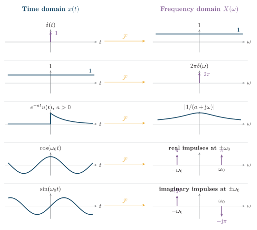
Common Fourier-transform pairs under the angular-frequency convention.

The constant, sinusoid, and impulse rows are distributional; they do not arise from ordinary absolutely convergent integrals. Impulse labels specify area. The sine pair has weight $+\mathrm{j}\pi$ at $-\omega_0$ and $-\mathrm{j}\pi$ at $+\omega_0$, as required by imaginary odd symmetry.

Common Fourier-transform pairs shown in both domains. Impulse arrows denote spectral weight; the causal-exponential panel shows magnitude, and the sine spectrum uses upward and downward arrows for opposite imaginary coefficients.

Each row of the figure compares a signal with its spectrum. An impulse has a flat spectrum; a constant becomes an impulse at $\omega=0$; a causal decaying exponential has a smooth low-pass magnitude; and the cosine and sine have line spectra at $\pm\omega_0$. The cosine lines are real, whereas the sine lines are purely imaginary with opposite signs.

Note

Example — Transform of a Rectangular Pulse

Let

$$x(t)=A\operatorname{rect}\!\left(\frac{t}{T_p}\right) = \begin{cases} A, & |t|<T_p/2,\\ 0, & |t|>T_p/2, \end{cases}$$

where endpoint values do not affect the integral. Then

$$\begin{aligned} X(\omega) &=A\int_{-T_p/2}^{T_p/2}e^{-\mathrm{j}\omega t}\,\mathrm{d}t\\ &=\frac{2A\sin(\omega T_p/2)}{\omega}\\ &=AT_p\operatorname{sinc}\!\left(\frac{\omega T_p}{2\pi}\right), \end{aligned}$$

with limiting value $X(0)=AT_p$, equal to the pulse area. The first zeros are at

$$\omega=\pm\frac{2\pi}{T_p},$$

so the two-sided null-to-null main-lobe width is $4\pi/T_p$ rad/s. In cyclic frequency the pair is

$$A\operatorname{rect}(t/T_p)\longleftrightarrow AT_p\operatorname{sinc}(fT_p),$$

with first zeros at $f=\pm1/T_p$ and null-to-null width $2/T_p$ hertz. Thus a shorter pulse has a wider spectrum, while a longer pulse has a narrower spectrum.

The pulse illustrates time–frequency spectral-width duality. More generally, replacing $x(t)$ by $x(at)$ compresses duration by $|a|$, expands spectral features by $|a|$, and scales spectral amplitude by $1/|a|$. Do not mix normalized $\operatorname{sinc}(\xi)=\sin(\pi\xi)/(\pi\xi)$ with the unnormalized function $\sin z/z$, whose zeros occur at nonzero multiples of $\pi$.

Application to LTI Systems

If an LTI system has impulse response $h(t)$ and frequency response $H(\omega)=\mathcal{F}\!\left\{h(t)\right\}$, then

Caution

Key Formula — LTI convolution and frequency response

$$y(t)=x(t)*h(t) \quad\Longleftrightarrow\quad Y(\omega)=X(\omega)H(\omega).$$

Thus

$$|Y(\omega)|=|X(\omega)|\,|H(\omega)|, \qquad \angle Y(\omega)=\angle X(\omega)+\angle H(\omega).$$

The system scales and phase-shifts each complex-exponential component independently. For a real LTI system, at a frequency where the steady-state response exists,

Caution

Key Formula — Sinusoidal steady-state response

$$A\cos(\omega_0t+\phi) \longrightarrow A|H(\omega_0)| \cos\!\left(\omega_0t+\phi+\angle H(\omega_0)\right).$$

This is the basis of filter analysis: $|H|$ sets passband gain and attenuation, while $\angle H$ sets phase distortion or delay. The convolution theorem replaces an integral with multiplication, and the frequency-shift property explains how modulation moves a baseband spectrum to a carrier frequency.

For an energy signal, Parseval gives the output energy directly:

$$E_y=\frac{1}{2\pi}\int_{-\infty}^{\infty} |X(\omega)|^2|H(\omega)|^2\,\mathrm{d}\omega.$$

Only frequencies present in the input contribute, so filter requirements need to hold over the occupied signal band rather than over all frequencies.

Exam Traps and Rapid Review

Tip

Exam Focus — Frequent Fourier mistakes

• State the frequency convention first. With angular frequency, the inverse contains $1/(2\pi)$; with cyclic frequency $f$, the kernel is $e^{-\mathrm{j}2\pi ft}$ and that inverse factor is absent.

• Do not mix the $a_0$ and $a_0/2$ trigonometric-series conventions. Here $a_0=C_0$ is the average value.

• A real signal requires positive- and negative-frequency complex lines. A one-sided sinusoidal amplitude is $2|C_n|$ for $n>0$.

• Periodic CT signals have discrete line spectra and generalized Fourier transforms made of impulses. A typical aperiodic energy signal has a continuous spectrum.

• Gibbs overshoot approaches about $9\%$ of the jump height. Its width shrinks, but its limiting fractional peak does not vanish.

• The transform of $x(t-t_0)$ is $e^{-\mathrm{j}\omega t_0}X(\omega)$. A delay changes phase, not magnitude.

• Time scaling requires $1/|a|$, not $1/a$; the absolute value accounts for reversal when $a<0$.

• Convolution in time gives direct multiplication, while multiplication in time gives frequency convolution with the factor $1/(2\pi)$.

• Distinguish normalized $\sin(\pi\xi)/(\pi\xi)$ from unnormalized $\sin z/z$ before quoting a rectangular-pulse pair.

• Absolute integrability is sufficient, not necessary. Constants, sinusoids, and impulses require generalized transforms.

[!NOTE]

Key Point — Fourier essentials

• Fourier series represents a periodic signal by coefficients at $\omega=n\omega_0$; Fourier transform represents a typical aperiodic signal by a continuous spectral density.

• Even symmetry removes sine terms, odd symmetry removes DC and cosine terms, and half-wave symmetry removes even harmonics.

• At a jump, a Fourier series converges to the midpoint and exhibits the Gibbs phenomenon.

• $\delta(t)\leftrightarrow1$, while duality gives $1\leftrightarrow2\pi\delta(\omega)$.

• Time convolution becomes frequency multiplication, yielding $Y(\omega)=X(\omega)H(\omega)$ for an LTI system.

• Parseval equates time-domain energy with $(1/2\pi)\int|X(\omega)|^2\,\mathrm{d}\omega$ and periodic average power with $\sum|C_n|^2$.