Electrostatics, Potential and Boundary Equations

Charge and Charge Density

Note

Electric charge and charge density.

Electric charge is the source of electrostatic fields. Line charge density $\lambda_l$, surface charge density $\rho_s$ and volume charge density $\rho_v$ specify charge per unit length, area and volume, respectively.

For continuous distributions,

$$dq=\lambda_l\,dl=\rho_s\,dS=\rho_v\,dV,$$

where $\lambda_l$ is line charge density, $\rho_s$ is surface charge density and $\rho_v$ is volume charge density.

Total charge is found by integration:

$$Q=\int_L\lambda_l\,dl, \qquad Q=\int_S\rho_s\,dS, \qquad Q=\int_V\rho_v\,dV.$$

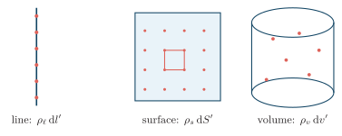
Charge element chosen from the source geometry.

Coulomb’s Law

Note

Coulomb’s law.

The electrostatic force between two point charges acts along their line of separation, is proportional to the product of the charges and is inversely proportional to the square of their distance.

For two point charges,

$$\mathbf{F}_{12}=\frac{1}{4\pi\varepsilon} \frac{q_1q_2}{R_{12}^2}\mathbf{a}_{12}.$$

$\mathbf{a}_{12}$ points from the source charge to the field point. Forces from multiple charges add by superposition.

For point charges $Q_i$ at positions $\mathbf r_i$, the field at $\mathbf r$ is therefore the vector sum

$$\mathbf E(\mathbf r)=\frac{1}{4\pi\varepsilon} \sum_i Q_i\frac{\mathbf r-\mathbf r_i} {\lvert\mathbf r-\mathbf r_i\rvert^3}.$$

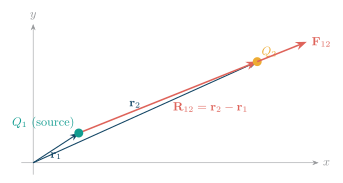
Displacement vector from source point to field point.

Electric Field Intensity

Note

Electric field intensity.

Electric field intensity $\mathbf E$ is the force exerted per unit positive test charge at a point.

$$\mathbf{E}=\frac{\mathbf{F}}{q}.$$

• Its SI unit is newton per coulomb ($\mathrm{N/C}$), equivalently volt per meter ($\mathrm{V/m}$).

• The force on a stationary charge is $\mathbf F=q\mathbf E$, so $\mathbf E$ gives both the physical force strength and the force direction for a positive test charge.

• For a fixed free-charge arrangement, changing the surrounding dielectric can change $\mathbf E$ because the material polarizes.

For a point charge,

$$\mathbf{E}=\frac{Q}{4\pi\varepsilon R^2}\mathbf{a}_R.$$

For a continuous charge distribution,

$$\mathbf{E}=\frac{1}{4\pi\varepsilon} \int \frac{\mathbf{R}}{R^3}\,dq.$$

$\mathbf{R}$ is always the displacement vector from the source element to the field point.

Note

Point charge in free space

For $Q=1\ \mu\mathrm C$ and $r=2\ \mathrm m$,

$$E=\frac{Q}{4\pi\varepsilon_0r^2} =\frac{(9\times10^9)(10^{-6})}{2^2} =2250\ \mathrm{V/m}.$$

The field is radially outward because the source charge is positive.

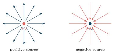
Electric field lines begin on positive charge and end on negative charge.

Infinite Line Charge

Let a uniform line charge $\lambda_l$ lie on the $z$-axis. At a point a radial distance $\rho$ from the line, an element $dq=\lambda_l\,dz'$ produces

$$d\mathbf E=\frac{\lambda_l\,dz'}{4\pi\varepsilon} \frac{\rho\mathbf a_\rho-z'\mathbf a_z} {(\rho^2+z'^2)^{3/2}}.$$

Elements at $+z'$ and $-z'$ cancel in the $z$-direction. Hence

$$\begin{aligned} \mathbf E & =\frac{\lambda_l\rho}{4\pi\varepsilon}\mathbf a_\rho \int_{-\infty}^{\infty}\frac{dz'}{(\rho^2+z'^2)^{3/2}} \\ & =\boxed{\frac{\lambda_l}{2\pi\varepsilon\rho}\mathbf a_\rho}. \end{aligned}$$

The $1/\rho$ dependence reflects cylindrical spreading of the flux.

Infinite Sheet Charge

For a uniform sheet $\rho_s$ in the $xy$-plane, symmetry cancels all components parallel to the sheet. Divide it into annular elements $dq=\rho_s2\pi\rho\,d\rho$. At $z>0$, their normal components give

$$E_z=\frac{\rho_s z}{2\varepsilon} \int_0^\infty\frac{\rho\,d\rho}{(\rho^2+z^2)^{3/2}} =\frac{\rho_s}{2\varepsilon}.$$

Thus

$$\mathbf E= \begin{cases} \dfrac{\rho_s}{2\varepsilon}\mathbf a_z, & z>0, \\[0.6em] -\dfrac{\rho_s}{2\varepsilon}\mathbf a_z, & z<0. \end{cases}$$

The ideal infinite-sheet field is independent of distance. Two oppositely charged parallel sheets therefore give $E=\rho_s/\varepsilon$ between them and zero field outside, when fringing is neglected.

Uniformly Charged Ring

For a continuous charge distribution, symmetry identifies which vector components cancel before integration. Consider a ring of radius $a$, total charge $Q$, and an observation point a distance $z$ along its axis.

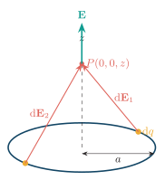
Only axial components add for a uniformly charged ring on its axis.

Every source element is at distance $R=\sqrt{a^2+z^2}$. Opposite elements cancel transversely, while their axial components add:

$$dE_z=\frac{z\,dq}{4\pi\varepsilon(a^2+z^2)^{3/2}}.$$

Since $\int dq=Q$,

$$\boxed{\mathbf E(0,0,z)= \frac{Qz}{4\pi\varepsilon(a^2+z^2)^{3/2}}\mathbf a_z}.$$

The field is zero at the ring centre. Far from the ring, $z\gg a$, it approaches the field of a point charge $Q$.

Electric Flux Density

Note

Electric flux density and electric flux.

Electric flux density $\mathbf D$, also called the electric displacement field, measures electric flux per unit area. It is especially useful because its closed-surface flux is determined by enclosed free charge.

In a general dielectric,

$$\mathbf D=\varepsilon_0\mathbf E+\mathbf P,$$

where $\mathbf P$ is the polarization density. For a linear, homogeneous and isotropic dielectric, this becomes

$$\mathbf{D}=\varepsilon\mathbf{E}.$$

The electric flux through a surface $S$ is

$$\Psi=\int_S\mathbf{D}\cdot d\mathbf{S}.$$

If $\mathbf D$ is uniform and normal to a flat area $A$, then

$$D=\frac{\Psi}{A}.$$

Thus $\mathbf D$ has SI unit coulomb per square meter ($\mathrm{C/m^2}$), while $\Psi$ has unit coulomb ($\mathrm C$).

• $\mathbf E$ is the physical force field and reflects the response of the medium, whereas $\mathbf D$ organizes the same electrostatic problem around free source charge.

• With a homogeneous medium and sufficient symmetry, Gauss’s law determines $\mathbf D$ from the free charge without using $\varepsilon$, and then $\mathbf E=\mathbf D/\varepsilon$.

• However, $\mathbf D$ is not universally independent of the medium. In inhomogeneous or anisotropic dielectric arrangements, material boundaries and constitutive properties can also affect its distribution.

Feature	Electric field $\mathbf E$	Flux density $\mathbf D$
Core idea	Force per unit positive test charge	Flux per unit area
Definition	$\mathbf F/q$	$\varepsilon_0\mathbf E+\mathbf P$
SI unit	$\mathrm{N/C}$ or $\mathrm{V/m}$	$\mathrm{C/m^2}$
Medium effect	Changes with material response	See constitutive law above
Source focus	Physical field at a point	Free charge through Gauss’s law
Main law	Coulomb’s law; $\mathbf E=-\nabla V$	Gauss’s law

Further reading: electric flux.

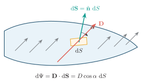
Flux through an arbitrarily oriented surface element.

Gauss’s Law

Note

Gauss’s law.

The net outward electric flux through any closed surface equals the free charge enclosed by that surface.

Integral form:

$$\oint_S\mathbf{D}\cdot d\mathbf{S}=Q_{\text{enc}}.$$

Using the divergence theorem,

$$\nabla\cdot\mathbf{D}=\rho_v.$$

This is Maxwell’s equation for electric flux from charge.

Enclosed Charge and Net Flux

The closed-surface diagram illustrates how charge is counted in Gauss’s law:

• $Q_{\text{enc}}$ is the algebraic sum of free charge inside the Gaussian surface. Here, $+q+q-q=+q$.

• A charge outside the surface can change $\mathbf D$ at individual points, but its total contribution to the closed-surface flux is zero.

• $d\mathbf S$ points outward. Outward field contributes positive flux and inward field contributes negative flux.

• The shape of the closed surface does not change the net flux; only $Q_{\text{enc}}$ does.

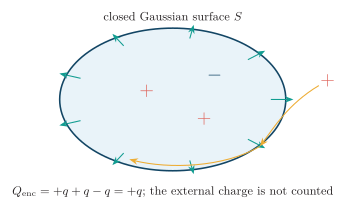
Closed-surface flux depends only on enclosed free charge.

Choosing the Gaussian Geometry

Choose a Gaussian surface that follows the symmetry of the source so that $\mathbf D\cdot d\mathbf S$ is constant or zero on each part of the surface:

• Spherical symmetry: for a point charge or a spherically symmetric charge distribution, $\mathbf D=D_r(r)\mathbf a_r$. It is normal and constant on a sphere, so $\oint_S\mathbf D\cdot d\mathbf S=D_r(4\pi r^2)$.

• Cylindrical symmetry: for an infinite line charge or a very long coaxial structure, $\mathbf D=D_\rho(\rho)\mathbf a_\rho$. Flux crosses only the curved surface, giving $D_\rho(2\pi\rho L)$; the end-cap flux is zero.

• Planar symmetry: for an infinite charged sheet, $\mathbf D$ is normal to the sheet and constant over each pillbox face. The side-wall flux is zero, and a two-sided sheet gives total flux $2DA$.

• Without sufficient symmetry, Gauss’s law remains true but does not by itself determine the field at each point on the surface.

The first three choices immediately give

$$\mathbf D_{\text{line}}=\frac{\lambda_l}{2\pi\rho}\mathbf a_\rho, \qquad \mathbf D_{\text{sheet}}=\frac{\rho_s}{2}\mathbf a_n, \qquad \mathbf D_{\text{point}}=\frac{Q}{4\pi r^2}\mathbf a_r.$$

Coulomb’s law sums contributions from the complete source distribution and is valid for arbitrary geometry. Gauss’s law instead uses only enclosed charge, but it becomes a direct field-calculation method only when symmetry makes the field direction known and its magnitude constant over the active parts of the Gaussian surface.

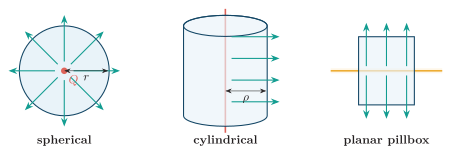
Gaussian surfaces chosen to match source symmetry.

Uniformly Charged Solid Sphere

For a sphere of radius $a$ with uniform volume charge density $\rho_v$:

• Inside, $r<a$: the enclosed charge grows as $r^3$, $Q_{\text{enc}}=\rho_v(4\pi r^3/3)$. Therefore $D_r(4\pi r^2)=Q_{\text{enc}}$, so $D_r=\rho_v r/3$ and the graph rises linearly from the centre.

• Outside, $r\ge a$: the entire charge $Q=\rho_v(4\pi a^3/3)$ is enclosed. Thus $D_r=\rho_v a^3/(3r^2)$, so the field falls as $1/r^2$.

• At $r=a$: both expressions give $D_r=\rho_v a/3$. The normal flux density is continuous because there is no free surface-charge sheet at the boundary.

• For positive $\rho_v$, $\mathbf D=D_r\mathbf a_r$ points radially outward.

For comparison, a thin spherical shell of radius $a$ and total charge $Q$ encloses no charge when $r<a$, so its internal field is zero. Outside the shell, it has the same field as a point charge at the centre:

$$\mathbf E= \begin{cases} 0, & r<a, \\[0.4em] \dfrac{Q}{4\pi\varepsilon r^2}\mathbf a_r, & r>a. \end{cases}$$

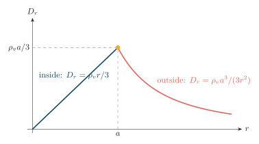
Flux density of a uniformly charged solid sphere.

Long Coaxial Cable

For a long coaxial cable with inner-conductor radius $a$, outer-conductor inner radius $b$, and inner line charge density $\lambda_l$:

• In the dielectric region $a<\rho<b$, choose a coaxial Gaussian cylinder of radius $\rho$ and length $L$.

• Cylindrical symmetry makes $\mathbf D=D_\rho(\rho)\mathbf a_\rho$ constant on the curved surface. It is tangential to the two end caps, so their flux is zero.

• Since $Q_{\text{enc}}=\lambda_lL$, $D_\rho(2\pi\rho L)=\lambda_lL$ and therefore $\mathbf D=\lambda_l\mathbf a_\rho/(2\pi\rho)$.

• The electric field in the dielectric is $\mathbf E=\mathbf D/\varepsilon$. It is zero inside either perfect conductor; outside an ideal coax carrying equal and opposite conductor charges, the net enclosed charge is zero.

• The result assumes a sufficiently long cable so that end fringing can be neglected.

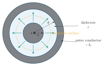
Gaussian cylinder for a long coaxial cable.

Standard Symmetry Results

Source	Field magnitude	Direction
Point charge $Q$	$E=\dfrac{Q}{4\pi\varepsilon r^2}$	radial
Infinite line charge $\lambda_l$	$E=\dfrac{\lambda_l}{2\pi\varepsilon\rho}$	outward cylindrical radial
Infinite sheet charge $\rho_s$	$E=\dfrac{\rho_s}{2\varepsilon}$	normal to sheet
Conducting surface	$D_n=\rho_s$ just outside	normal to conductor

Electric Potential

Note

Electric potential.

Electric potential is the electric potential energy per unit positive test charge, $V=U/q_0$. Equivalently, it is the external work per unit charge required to bring $q_0$ slowly from a chosen reference point without changing its kinetic energy. It is a scalar field, independent of $q_0$, that describes the electrical energy landscape produced by the sources and medium. Its SI unit is the volt: $1\ \mathrm{V}=1\ \mathrm{J/C}$.

For slow motion from $A$ to $B$,

$$V_B-V_A =\frac{U_B-U_A}{q_0} =\frac{W_{\mathrm{ext},A\to B}}{q_0} =-\frac{W_{\mathrm{field},A\to B}}{q_0} =-\int_A^B\mathbf E\cdot d\mathbf l.$$

• A positive charge moving along $\mathbf E$ loses potential; moving against $\mathbf E$ requires positive external work and raises its potential.

• Only potential differences are physical: adding a constant to $V$ does not change $\mathbf E$.

For a localized charge distribution, infinity may be chosen as the reference because the potential approaches zero there:

$$V(\infty)=0, \qquad V(\mathbf r)=-\int_{\infty}^{\mathbf r}\mathbf E\cdot d\mathbf l.$$

Once the reference is fixed, $V$ is uniquely determined.

For a point charge, substituting its radial field into the potential integral gives

$$V(r)=-\int_\infty^r\frac{Q}{4\pi\varepsilon R^2}\,dR =\boxed{\frac{Q}{4\pi\varepsilon r}}.$$

Field-Potential Relation

Electrostatic work is path independent. By Stokes’ theorem,

$$\oint_C\mathbf E\cdot d\mathbf l =\int_S(\nabla\times\mathbf E)\cdot d\mathbf S=0, \qquad \nabla\times\mathbf E=0.$$

This is Faraday’s law with no time-varying magnetic flux. Therefore the curl-free field is the negative gradient of potential:

$$\boxed{\mathbf E=-\nabla V} =-\left( \mathbf a_x\frac{\partial V}{\partial x} +\mathbf a_y\frac{\partial V}{\partial y} +\mathbf a_z\frac{\partial V}{\partial z} \right).$$

Thus $\mathbf E$ points along the steepest decrease of $V$; a rapid spatial change in $V$ means a strong field.

Potential of Charge Distributions

In a homogeneous medium of permittivity $\varepsilon$, with $V(\infty)=0$,

$$V_Q=\frac{Q}{4\pi\varepsilon R}, \qquad V(\mathbf r)=\frac{1}{4\pi\varepsilon}\sum_i\frac{Q_i}{R_i}.$$

Potential is positive for $Q>0$, negative for $Q<0$, and contributions add algebraically because $V$ is scalar.

For a continuous distribution, $\mathbf r'$ locates the source element, $\mathbf r$ the observation point, and $R=\lvert\mathbf r-\mathbf r'\rvert$:

$$V(\mathbf r)=\frac{1}{4\pi\varepsilon}\int\frac{dq}{R},$$

or, according to source geometry,

$$V(\mathbf r)=\frac{1}{4\pi\varepsilon} \begin{cases} \displaystyle\int_L\frac{\lambda_l(\mathbf r')}{R}\,dl', & \text{line charge}, \\[1.1em] \displaystyle\int_S\frac{\rho_s(\mathbf r')}{R}\,dS', & \text{surface charge}, \\[1.1em] \displaystyle\int_{\mathcal V}\frac{\rho_v(\mathbf r')}{R}\,dV', & \text{volume charge}. \end{cases}$$

Equipotential Surfaces

Note

Equipotential surface.

An equipotential surface is a locus of points having the same electric potential, $V=\text{constant}$.

$$V_B-V_A=0, \qquad W_{\mathrm{field}}=-q(V_B-V_A)=0, \qquad dV=-\mathbf E\cdot d\mathbf l =-E\,dl\cos\theta=0.$$

Since $E\ne0$ and $dl\ne0$, $\cos\theta=0$ and therefore $\theta=90^\circ$. Hence $\mathbf E$ is normal to every equipotential surface.

Properties

• The tangential electric-field component is zero: $E_t=0$.

• Two equipotential surfaces cannot intersect, because one point cannot have two different potential values.

• The surface of a perfect conductor in electrostatic equilibrium is an equipotential surface.

Common geometries

• Point charge: concentric spherical surfaces, with $V\propto 1/r$.

• Infinite line charge or coaxial cable: concentric cylindrical surfaces.

• Uniform parallel field: parallel planes perpendicular to the electric-field direction.

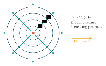
Equipotential surfaces are normal to electric field lines.

Parallel plates. Between ideal parallel plates, $\mathbf E$ is approximately uniform away from the edges; equipotentials are parallel to the plates and perpendicular to $\mathbf E$. For separation $d$,

$$\lvert\Delta V\rvert=Ed.$$

The potential varies linearly along the field direction, and every path between the same endpoints gives the same potential difference.

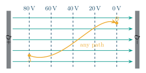
Parallel-plate equipotentials and path-independent potential difference.

Energy and Capacitance

Note

Electrostatic energy density and capacitance.

• Electrostatic energy density $w_e$ is electric-field energy stored per unit volume.

• Capacitance $C$ is the charge stored per unit potential difference, $C=Q/V$.

Electrostatic energy density is

$$w_e=\frac{1}{2}\mathbf{E}\cdot\mathbf{D} =\frac{1}{2}\varepsilon E^2.$$

Total stored energy is

$$W_e=\frac{1}{2}\int_V\varepsilon E^2\,dV.$$

For a capacitor,

$$C=\frac{Q}{V}, \qquad W=\frac{1}{2}CV^2=\frac{Q^2}{2C}=\frac{1}{2}QV.$$

The energy relation follows by charging the capacitor gradually. When the instantaneous charge is $q$, its voltage is $v=q/C$, so the incremental work is $dW=v\,dq$. Therefore

$$W=\int_0^Q\frac{q}{C}\,dq =\frac{Q^2}{2C} =\frac{1}{2}QV =\frac{1}{2}CV^2.$$

Expressing this energy as an integral over the field volume gives $W_e=\int_V w_e\,dV$, with

$$\boxed{w_e=\frac{1}{2}\mathbf E\cdot\mathbf D}.$$

Conductors and Electrostatic Boundaries

Perfect Conductor Boundary

Note

Perfect conductor in electrostatic equilibrium.

A perfect conductor in electrostatic equilibrium has zero internal electric field, constant potential throughout its volume and surface, and no tangential electric field at its boundary.

• Inside the conductor: Free charges redistribute until the static internal field becomes zero, $\mathbf E=0$. Since $\mathbf E=-\nabla V$, it follows that $\nabla V=0$ and the conductor has constant potential throughout its volume and surface.

• Tangential component: At the boundary, $E_t=0$. Any nonzero tangential field would exert a force on free surface charges, causing them to move until electrostatic equilibrium was restored.

• Normal component: The field immediately outside is perpendicular to the surface, $\mathbf E_{\mathrm{out}}=E_n\mathbf a_n$, where $\mathbf a_n$ is the outward unit normal.

• Surface-charge relation: A Gaussian pillbox across the surface gives $D_n=\rho_s$ immediately outside. In a linear dielectric, $E_n=\rho_s/\varepsilon$.

The conductor diagram below shows the zero tangential component, the outward normal, and the normal exterior field at a curved surface.

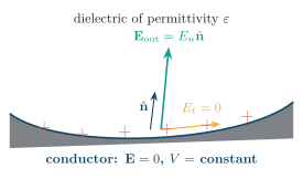
Electrostatic field at a conductor surface.

Polarization and Bound Surface Charge

An applied field aligns dielectric dipoles and produces polarization $\mathbf P$. For a dielectric with outward unit normal $\mathbf a_n$, the bound surface-charge density is

$$\rho_{sb}=\mathbf P\cdot\mathbf a_n=P_n.$$

• The face from which $\mathbf P$ emerges carries $\rho_{sb}=+P_n$.

• The opposite face carries $\rho_{sb}=-P_n$.

• For uniform polarization, the opposite bound charges are equal and the dielectric remains neutral overall.

The polarization diagram below connects the aligned dipoles to the signs of the bound charge on the two faces.

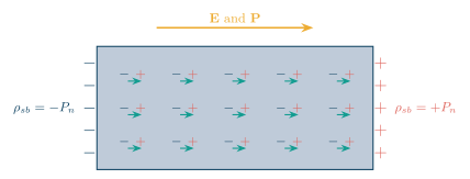
Bound surface charge on a polarized dielectric.

Dielectric-Dielectric Boundary

Note

Electrostatic dielectric boundary conditions.

At an interface, tangential electric field is continuous, while the normal electric flux density changes by the free surface charge density $\rho_s$.

Let $\mathbf a_n$ point from medium 1 to medium 2, and denote free surface charge by $\rho_{sf}$. Then,

$$\mathbf{a}_n\times(\mathbf{E}_2-\mathbf{E}_1)=0, \qquad \mathbf{a}_n\cdot(\mathbf{D}_2-\mathbf{D}_1)=\rho_{sf}.$$

Thus $E_{1t}=E_{2t}$. At a charge-free interface, $\rho_{sf}=0$, so $D_{1n}=D_{2n}$ and, for linear media,

$$\varepsilon_1E_{1n}=\varepsilon_2E_{2n}.$$

If $\theta_1$ and $\theta_2$ are measured from the normal, these component conditions give

$$\frac{\tan\theta_1}{\tan\theta_2}=\frac{\varepsilon_1}{\varepsilon_2}.$$

The refraction diagram below shows the continuous tangential component and the permittivity-dependent change in the normal electric-field component.

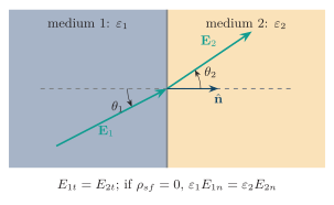
Electrostatic field refraction at a charge-free dielectric boundary.

Poisson and Laplace Equations

Note

Poisson and Laplace equations.

Poisson’s equation relates potential curvature to volume charge density, $\nabla^2V=-\rho_v/\varepsilon$ for uniform $\varepsilon$; Laplace’s equation, $\nabla^2V=0$, is its charge-free form.

Poisson’s equation follows from Gauss’s law in differential form, one of Maxwell’s equations,

$$\nabla\cdot\mathbf{D}=\rho_v.$$

For a linear, homogeneous medium, $\mathbf{D}=\varepsilon\mathbf{E}$ with constant $\varepsilon$. In electrostatics, $\mathbf{E}=-\nabla V$. Substitution gives

$$\nabla\cdot\mathbf{D} =\nabla\cdot\left(-\varepsilon\nabla V\right) =\rho_v.$$

Since $\varepsilon$ is constant throughout the region,

$$-\varepsilon\nabla^2V=\rho_v, \qquad \nabla^2V=-\frac{\rho_v}{\varepsilon}.$$

This is Poisson’s equation. It is used to determine the potential when the region contains a known volume-charge distribution $\rho_v$. If the region is charge free, $\rho_v=0$, and Poisson’s equation reduces to Laplace’s equation,

$$\nabla^2V=0.$$

A charge-free region need not be field free: charges or fixed potentials on its boundaries can still produce a nonzero potential and electric field within it. After solving either equation with the appropriate boundary conditions, recover the field from $\mathbf{E}=-\nabla V$.

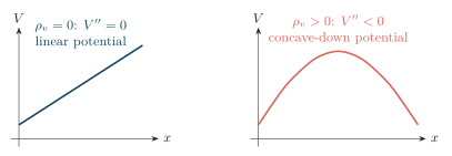
Potential curvature reveals local volume charge in one dimension.

Boundary-Value Problems

Note

Electrostatic boundary-value problem.

An electrostatic boundary-value problem determines potential $V$ from Poisson’s or Laplace’s equation and specified boundary data, then recovers the field from $\mathbf E=-\nabla V$.

Common boundary data are specified conductor potentials, known surface charge, dielectric interfaces and symmetry planes.

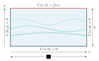
Rectangular Laplace problem for Cartesian separation of variables.

For two infinite plates at $x=0$ and $x=d$, let $V(0)=V_1$ and $V(d)=V_2$. With no fringing or volume charge, the potential depends only on $x$, so

$$\frac{d^2V}{dx^2}=0.$$

Two integrations give $V(x)=Ax+B$. Applying the two boundary values yields

$$\boxed{V(x)=V_1+\frac{V_2-V_1}{d}x}, \qquad 0\le x\le d,$$

and hence the uniform electric field

$$\boxed{\mathbf E=-\nabla V =\frac{V_1-V_2}{d}\mathbf a_x}.$$

The potential varies linearly and the field points from the higher-potential plate toward the lower-potential plate.

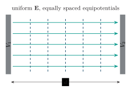
One-dimensional Laplace solution between fixed potentials.

For concentric conductors, spherical symmetry instead reduces the solution to a radial function.

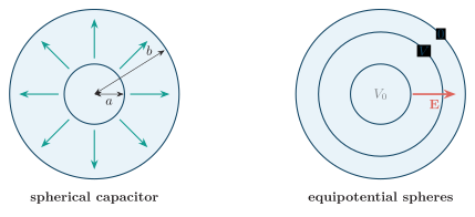
Concentric spherical conductors match spherical-coordinate symmetry.