System Stability and Sensitivity

Stability determines whether a control system can operate safely, while sensitivity and disturbance rejection quantify how robustly it preserves its intended behavior when the plant or its environment changes.

System Stability

A control system is stable when bounded operating signals do not produce an unbounded output and its unforced natural response does not grow with time. An asymptotically stable system has a natural response that decays to zero.

BIBO Stability

A system is bounded-input, bounded-output (BIBO) stable if every bounded input produces a bounded output. Thus, for finite constants $M_r$ and $M_c$,

$$|r(t)|\leq M_r<\infty \quad\Longrightarrow\quad |c(t)|\leq M_c<\infty$$

for all time.

Stability from Closed-Loop Poles

For a finite-dimensional continuous-time LTI system with no hidden unstable modes or unstable pole–zero cancellations, the closed-loop pole locations give the following test.

Law — Continuous-time pole test

Closed-loop pole location	System behavior
All poles strictly in the left half-plane	Asymptotically stable and BIBO stable.
At least one pole in the right half-plane	Unstable.
Only simple poles on the imaginary axis, with all others in the left half-plane	Marginally stable in the zero-input sense; generally not BIBO stable.
A repeated pole on the imaginary axis	Unstable because the natural response contains growing terms.

The imaginary-axis qualification matters: a simple undamped mode can have a bounded natural response, yet a bounded sinusoid at resonance can produce an unbounded forced response. It is therefore called marginal rather than asymptotically stable.

Absolute and Relative Stability

Absolute stability answers the yes-or-no question of whether the system is stable. Relative stability describes how close it is to instability and how rapidly transients decay. Common measures are:

• the distance of dominant poles from the imaginary axis;

• damping ratio $\zeta$ and settling time;

• gain margin; and

• phase margin.

Characteristic Equation

For the standard negative-feedback system,

Caution

Key Formula — Characteristic equation

$$T(s)=\frac{C(s)}{R(s)}=\frac{G(s)}{1+G(s)H(s)}, \qquad \boxed{1+G(s)H(s)=0}.$$

The roots of the characteristic equation are the closed-loop poles and decide closed-loop stability.

The Routh–Hurwitz criterion tests whether a characteristic polynomial has right-half-plane roots directly from its coefficients, without explicitly solving for every root.

Tip

Exam Focus — Feedback and stability

Negative feedback improves stability only when the loop has adequate gain and phase margins. The sign at the summing junction alone is not a stability proof; the characteristic equation must be tested.

Sensitivity

The sensitivity of a transfer function $T$ to a parameter $K$ is the ratio of their fractional changes:

$$\boxed{S_K^T =\frac{\partial T/T}{\partial K/K} =\frac{K}{T}\frac{\partial T}{\partial K}}.$$

For a small parameter change, $\Delta T/T\approx S_K^T\,\Delta K/K$.

Sensitivity is generally a function of frequency and may be complex. Its magnitude indicates how strongly relative parameter error is transmitted to the closed-loop transfer function.

Sensitivity to Forward-Path Gain

For negative feedback, hold $H$ fixed and write

$$T=\frac{G}{1+GH}.$$

Then

$$\begin{aligned} \frac{\partial T}{\partial G} &=\frac{(1+GH)-GH}{(1+GH)^2} =\frac{1}{(1+GH)^2},\\ \frac{G}{T}&=1+GH. \end{aligned}$$

Therefore,

Caution

Key Formula — Forward-path sensitivity

$$\boxed{S_G^T =\frac{G}{T}\frac{\partial T}{\partial G} =\frac{1}{1+GH}} =\frac{1}{1+L}.$$

For an open-loop system $T=G$, so $S_G^T=1$. At frequencies where the negative-feedback loop gain is positive real, feedback reduces forward-path sensitivity by the factor $1+GH$. More generally, the reduction is governed by $|1+L(j\omega)|$, and it is lost near the critical point $L=-1$.

Sensitivity to the Feedback Element

Now hold $G$ fixed. Differentiation gives

$$\begin{aligned} \frac{\partial T}{\partial H} &=-\frac{G^2}{(1+GH)^2},\\ \frac{H}{T}&=\frac{H(1+GH)}{G}. \end{aligned}$$

Hence,

Caution

Key Formula — Feedback-element sensitivity

$$\boxed{S_H^T =\frac{H}{T}\frac{\partial T}{\partial H} =-\frac{GH}{1+GH}} =-\frac{L}{1+L}.$$

If $|GH|\gg 1$ away from $L=-1$, then $S_H^T\approx-1$.

The negative sign means that a fractional increase in $H$ produces approximately the opposite fractional change in $T$ at high loop gain. Thus, large loop gain desensitizes the system to the forward path but makes the closed-loop scale depend directly on the accuracy and stability of the feedback element.

Disturbance Rejection

Consider an additive output disturbance $D(s)$ applied after the plant in a unity negative-feedback loop.

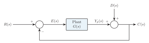
Signed output-disturbance loop with additive disturbance and unity negative feedback.

For the figure,

$$\begin{aligned} E(s)&=R(s)-C(s),\\ Y_p(s)&=G(s)E(s),\\ C(s)&=Y_p(s)+D(s). \end{aligned}$$

Therefore,

$$\begin{aligned} C(s)&=G(s)\bigl[R(s)-C(s)\bigr]+D(s),\\ \bigl[1+G(s)\bigr]C(s)&=G(s)R(s)+D(s). \end{aligned}$$

Caution

Key Formula — Reference and output-disturbance responses

$$\boxed{C(s) =\frac{G(s)}{1+G(s)}R(s) +\frac{1}{1+G(s)}D(s)}.$$

With the reference set to zero,

$$\boxed{\left.\frac{C(s)}{D(s)}\right|_{R=0} =\frac{1}{1+G(s)}}.$$

Thus high loop gain suppresses an output disturbance at frequencies where $|G(j\omega)|$ is large and the closed loop remains stable. Disturbances injected at other points have different transfer functions, so the injection location must always be identified before writing a rejection factor.

Control-System Components

Error Detector

An error detector compares the reference and feedback signals. Practical examples include a potentiometer pair in position control, a synchro pair in AC position control, and a differential amplifier in electronic control.

Controller

The controller processes the error and produces the command applied to the plant or actuator.

Controller	Transfer function	Main effect
P	$K_p$	Speeds response and reduces error, but may leave steady-state error.
I	$K_i/s$	Eliminates steady-state error, but can reduce stability margins.
D	$K_d s$	Predictive action that improves damping.
PI	$K_p+K_i/s$	Combines proportional response with zero steady-state error.
PD	$K_p+K_d s$	Improves damping and transient response.
PID	$K_p+K_i/s+K_d s$	Combines steady-state accuracy with transient damping.

Common ideal controller actions.

Ideal derivative action amplifies high-frequency measurement noise and is therefore implemented with filtering in practical controllers.

Actuator

An actuator converts the controller output into physical action and supplies the energy needed to drive the plant. Examples are DC motors, hydraulic and pneumatic actuators, solenoid valves, and power amplifiers.

Sensor

A sensor measures the controlled output or another system state. Typical pairings are:

Measured quantity	Sensor
Speed	Tachogenerator
Position	Potentiometer or encoder
Temperature	Thermocouple or resistance temperature detector (RTD)
Pressure	Pressure transducer

Typical feedback sensors.

Solved Examples

Note

Example — Closed-loop transfer function

A system has

$$G(s)=\frac{100}{s+10}, \qquad H(s)=0.1.$$

Find its negative-feedback closed-loop transfer function.

Solution.

$$\begin{aligned} T(s) &=\frac{G(s)}{1+G(s)H(s)}\\ &=\frac{\dfrac{100}{s+10}} {1+\dfrac{100}{s+10}(0.1)}\\ &=\frac{100}{s+10+10}. \end{aligned}$$

Thus,

$$\boxed{T(s)=\frac{100}{s+20}}.$$

[!NOTE]

Example — Sensitivity reduction

A closed-loop system has loop gain $GH=99$. Find the sensitivity of its closed-loop transfer function to a forward-gain variation.

Solution.

$$S_G^T=\frac{1}{1+GH} =\frac{1}{1+99} =\boxed{0.01}.$$

Consequently, a 10 % change in $G$ produces approximately a 0.1 % change in $T$ for a small variation about this operating condition.

Example — Stability from pole locations

Classify systems having the following closed-loop pole sets.

Poles	Classification	Reason
$-2,-5$	Stable	Every pole lies in the left half-plane.
$-1,+3$	Unstable	The pole at $+3$ lies in the right half-plane.
$\pm\mathrm{j}4$	Marginally stable	The imaginary-axis poles are simple; the system is not asymptotically stable and is generally not BIBO stable.
$0,0,-2$	Unstable	The origin is a repeated imaginary-axis pole.

Quick Revision Table

Topic	Key result
Open-loop system	Control action is independent of output.
Closed-loop system	Control action depends on output through feedback.
Negative-feedback transfer function	$T(s)=G(s)/[1+G(s)H(s)]$.
Positive-feedback transfer function	$T(s)=G(s)/[1-G(s)H(s)]$.
Loop gain	$L(s)=G(s)H(s)$.
Characteristic equation	$1+G(s)H(s)=0$ for the standard negative-feedback loop.
BIBO stability	Every bounded input produces a bounded output.
Stable pole condition	All closed-loop poles lie strictly in the left half-plane.
Forward-path sensitivity	$S_G^T=1/(1+GH)$.
Feedback-element sensitivity	$S_H^T=-GH/(1+GH)$.
Output-disturbance reduction	$C/D=1/(1+G)$ for the stated unity-feedback injection point.

Control-system fundamentals at a glance.

Note

Key Point — Quick review

• Open-loop systems are simple but cannot correct errors caused by disturbances or parameter changes.

• Closed-loop systems use feedback to reduce error and forward-path sensitivity.

• Negative feedback gives $S_G^T=1/(1+GH)$, subject to the loop remaining stable.

• The characteristic equation $1+G(s)H(s)=0$ determines the closed-loop poles.

• Asymptotic continuous-time stability requires every closed-loop pole to lie strictly in the left half-plane.