the roots zi and pi expose much of the input-output dynamics without solving the differential equation explicitly.
The zeros are roots of the numerator:
N(zi)=0.
For an uncancelled zero, G(zi)=0. Zeros weight and reshape the forced response, but zeros alone do not determine stability.
The poles are roots of the denominator:
D(pi)=0.
An uncancelled pole is a singularity of G(s) and contributes a natural mode of the form epit; a repeated pole contributes polynomial factors such as tepit.
The characteristic polynomial of the standard second-order system is
s2+2ζωns+ωn2=0.
For 0<ζ<1, its poles are
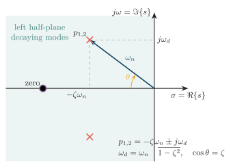
p1,2=−ζωn±jωd,ωd=ωn1−ζ2.
Thus the radial distance from the origin is ωn, the horizontal distance to the imaginary axis is ζωn, and the angle measured from the negative real axis satisfies cosθ=ζ.
Geometry of an underdamped second-order pole pair in the s-plane.
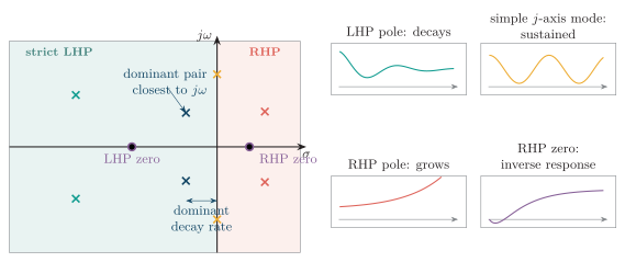
For a finite-dimensional, proper, continuous-time rational transfer function, BIBO stability requires every uncancelled pole to lie strictly in the open left half-plane. Pole location determines both the mode shape and its decay or growth.
Pole location
Natural-response term
Conclusion
Negative real axis
Decaying exponential e−at, a>0
Asymptotically decaying
Complex pair in LHP
Decaying sinusoid e−σtsinωt
Asymptotically decaying
Positive real axis
Growing exponential eat
Unstable
Complex pair in RHP
Growing sinusoid eσtsinωt
Unstable
Simple pole at origin
Constant natural mode; step input to an integrator gives a ramp
Not BIBO stable
Simple pair on jω axis
Sustained sinusoidal natural mode
Not BIBO stable; marginal only in the internal-mode sense
Repeated pole on jω axis
Polynomially growing oscillation
Unstable
Significance of continuous-time pole locations
Pole regions, dominant-pole distance, representative zeros, and their response signatures.
Zeros alter modal weights and frequency response rather than creating unforced modes. Depending on location and relative strength, a zero can speed the initial response, increase overshoot, or partially suppress a pole’s visible contribution. A right-half-plane zero is a non-minimum-phase zero; it commonly produces an initial motion in the wrong direction (undershoot or inverse response) and limits achievable feedback bandwidth.