Exam Focus
Be able to derive N A = n 1 2 − n 2 2 \mathrm{NA}=\sqrt{n_1^2-n_2^2} NA = n 1 2 − n 2 2 N A ≈ n 1 2 Δ \mathrm{NA}\approx n_1\sqrt{2\Delta} NA ≈ n 1 2Δ V-number V = 2 π a N A / λ V=2\pi a\,\mathrm{NA}/\lambda V = 2 π a NA / λ V < 2.405 V<2.405 V < 2.405
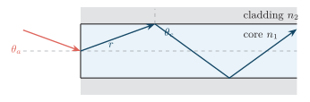
The acceptance angle θ a \theta_a θ a acceptance cone . The numerical aperture (NA) measures the fibre’s light-gathering ability, N A = n 0 sin θ a \mathrm{NA}=n_0\sin\theta_a NA = n 0 sin θ a
Limiting guided ray: refraction at the end face (n 0 sin θ a = n 1 sin r n_0\sin\theta_a=n_1\sin r n 0 sin θ a = n 1 sin r i = 90 ∘ − r = θ c i=90^\circ-r=\theta_c i = 9 0 ∘ − r = θ c
Key Point — NA derivation
At the flat end face, Snell’s law gives n 0 sin θ a = n 1 sin r n_0\sin\theta_a=n_1\sin r n 0 sin θ a = n 1 sin r i = 90 ∘ − r i=90^\circ-r i = 9 0 ∘ − r i = θ c i=\theta_c i = θ c sin θ c = n 2 / n 1 \sin\theta_c=n_2/n_1 sin θ c = n 2 / n 1 sin r = cos θ c = 1 − n 2 2 / n 1 2 \sin r=\cos\theta_c=\sqrt{1-n_2^2/n_1^2} sin r = cos θ c = 1 − n 2 2 / n 1 2
n 0 sin θ a = n 1 1 − n 2 2 n 1 2 ⇒ N A = n 0 sin θ a = n 1 2 − n 2 2 n_0\sin\theta_a=n_1\sqrt{1-\tfrac{n_2^2}{n_1^2}}
\;\Rightarrow\;
\boxed{\;\mathrm{NA}=n_0\sin\theta_a=\sqrt{n_1^2-n_2^2}\;} n 0 sin θ a = n 1 1 − n 1 2 n 2 2 ⇒ NA = n 0 sin θ a = n 1 2 − n 2 2 and in air (n 0 = 1 n_0=1 n 0 = 1 N A = sin θ a \mathrm{NA}=\sin\theta_a NA = sin θ a
[!IMPORTANT]
Key Formula — Relative index difference and weakly-guiding NA
Δ = n 1 − n 2 n 1 , N A ≈ n 1 2 Δ ( Δ ≪ 1 ) . \Delta=\frac{n_1-n_2}{n_1},\qquad
\mathrm{NA}\approx n_1\sqrt{2\Delta}\quad(\Delta\ll1). Δ = n 1 n 1 − n 2 , NA ≈ n 1 2Δ ( Δ ≪ 1 ) . [!NOTE]
Key Point — Significance of NA
Higher NA ⇒ \Rightarrow ⇒ ⇒ \Rightarrow ⇒
Key Formula — Normalised frequency (V-number)
V = 2 π a λ N A , V=\frac{2\pi a}{\lambda}\,\mathrm{NA}, V = λ 2 π a NA , a = a= a = λ = \lambda= λ =
Condition Result V < 2.405 V<2.405 V < 2.405 Single-mode (only the fundamental mode propagates) Step-index MMF M ≈ V 2 / 2 M\approx V^2/2 M ≈ V 2 /2 Graded-index MMF M ≈ V 2 / 4 M\approx V^2/4 M ≈ V 2 /4
Single-mode cut-off and approximate mode count.
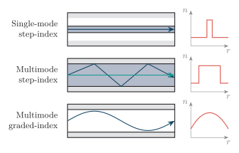
Fibres are classified by material (glass, plastic), index profile (step, graded) and number of modes (single, multi).
Fibre types: core sections/ray paths (left) and radial index profiles n ( r ) n(r) n ( r )
Feature Single-mode fibre (SMF) Multimode fibre (MMF) Core diameter ≈ 8 \approx 8 ≈ 8 10 μ m 10\,\mu\mathrm{m} 10 μ m 50 50 50 62.5 μ m 62.5\,\mu\mathrm{m} 62.5 μ m Modes One Many Modal dispersion Almost zero Significant Bandwidth× \times × Very high Lower Source Laser diode LED / VCSEL Coupling alignment Critical Easier Application Long-haul, FTTH backbone LAN, short reach
Single-mode versus multimode fibre.
Feature Step-index MMF Graded-index MMF Index profile Abrupt core–cladding step Gradual radial decrease Ray path Zig-zag Curved Modal dispersion High Lower Bandwidth Low Higher
Step-index versus graded-index multimode fibre.
Example — Numerical aperture and acceptance angle
n 1 = 1.50 n_1=1.50 n 1 = 1.50 n 2 = 1.47 n_2=1.47 n 2 = 1.47
N A = 1.50 2 − 1.47 2 = 2.25 − 2.1609 = 0.0891 ≈ 0.2985 , \mathrm{NA}=\sqrt{1.50^2-1.47^2}=\sqrt{2.25-2.1609}=\sqrt{0.0891}\approx\boxed{0.2985}, NA = 1.5 0 2 − 1.4 7 2 = 2.25 − 2.1609 = 0.0891 ≈ 0.2985 , θ a = sin − 1 ( 0.2985 ) ≈ 17.4 ∘ . \theta_a=\sin^{-1}(0.2985)\approx\boxed{17.4^\circ}. θ a = sin − 1 ( 0.2985 ) ≈ 17. 4 ∘ . [!NOTE]
Example — Single-mode test with the V-number
Core radius a = 4.5 μ m a=4.5\,\mu\mathrm{m} a = 4.5 μ m N A = 0.12 \mathrm{NA}=0.12 NA = 0.12 λ = 1.55 μ m \lambda=1.55\,\mu\mathrm{m} λ = 1.55 μ m
V = 2 π a λ N A = 2 π ( 4.5 ) ( 0.12 ) 1.55 ≈ 2.19. V=\frac{2\pi a}{\lambda}\mathrm{NA}=\frac{2\pi(4.5)(0.12)}{1.55}\approx2.19. V = λ 2 π a NA = 1.55 2 π ( 4.5 ) ( 0.12 ) ≈ 2.19. Since V < 2.405 V<2.405 V < 2.405 single-mode at this wavelength.