Z-Transform, Laplace Transform, and Sampling

The Z-transform and Laplace transform extend frequency-domain analysis by including a convergence factor. Their regions of convergence distinguish signals that can have the same algebraic transform, while sampling provides the bridge from continuous-time signals to discrete-time sequences.

Z-Transform

Definition and Region of Convergence

The bilateral Z-transform of a discrete-time sequence $x[n]$ is

$$X(z)=\mathcal{Z}\!\left\{x[n]\right\}=\sum_{n=-\infty}^{\infty}x[n]z^{-n}, \qquad z=re^{\mathrm{j}\Omega}.$$

Its region of convergence (ROC) is the set of complex values of $z$ for which this sum converges.

The ROC is part of the transform specification, not an optional annotation. For example, the same expression $1/(1-az^{-1})$ represents a right-sided or a left-sided sequence according to whether its ROC is outside or inside the pole at $z=a$. An algebraic expression without its ROC therefore does not uniquely identify the sequence.

Sequence	Z-transform	Region of convergence
$\delta[n]$	$1$	Entire $z$-plane
$u[n]$	$\dfrac{1}{1-z^{-1}}$	$\lvert z\rvert>1$
$a^n u[n]$	$\dfrac{1}{1-az^{-1}}$	$\lvert z\rvert>\lvert a\rvert$
$-a^n u[-n-1]$	$\dfrac{1}{1-az^{-1}}$	$\lvert z\rvert<\lvert a\rvert$

Common bilateral Z-transform pairs.

Properties and Value Theorems

If $x[n]\leftrightarrow X(z)$ and $y[n]\leftrightarrow Y(z)$, the principal properties are as follows.

Property	Time-domain operation	Z-domain result
Linearity	$\alpha x[n]+\beta y[n]$	$\alpha X(z)+\beta Y(z)$
Time shift	$x[n-n_0]$	$z^{-n_0}X(z)$
Convolution	$x[n]*y[n]$	$X(z)Y(z)$
Multiplication by $n$	$n x[n]$	$-z\dfrac{\mathrm{d}X(z)}{\mathrm{d}z}$
Time reversal	$x[-n]$	$X(z^{-1})$
Initial value	$x[0]$	$\displaystyle\lim_{z\to\infty}X(z)$
Final value	$\displaystyle\lim_{n\to\infty}x[n]$	$\displaystyle\lim_{z\to 1}(1-z^{-1})X(z)$

Important Z-transform properties.

The ROC must be reconsidered after every operation. In particular, pole-zero cancellation can alter an apparent ROC boundary, and time reversal maps the ROC by inversion.

Note

Key Point — Qualifications for the Z-transform value theorems

The initial-value theorem in the table assumes that $x[n]$ is causal. The final-value theorem applies only when $(1-z^{-1})X(z)$ has all its poles strictly inside the unit circle; equivalently, $X(z)$ may contain one simple pole at $z=1$, but every other pole relevant to the sequence must lie strictly inside the unit circle. A repeated pole at $z=1$, or any uncancelled pole on or outside the unit circle, invalidates the theorem. These conditions ensure that the limit $\lim_{n\to\infty}x[n]$ actually exists.

Derivation of a Standard Pair

For $x[n]=a^n u[n]$, only samples with $n\geq 0$ are present. Hence

$$\begin{aligned} X(z) &=\sum_{n=0}^{\infty}a^n z^{-n} =\sum_{n=0}^{\infty}(az^{-1})^n \\ &=\frac{1}{1-az^{-1}} =\frac{z}{z-a}. \end{aligned}$$

The geometric series converges only when

$$\lvert az^{-1}\rvert<1 \quad\Longleftrightarrow\quad \lvert z\rvert>\lvert a\rvert.$$

Therefore the complete transform pair is

Caution

Key Formula — Causal exponential sequence

$$a^n u[n]\ \leftrightarrow\ \frac{1}{1-az^{-1}}, \qquad \text{ROC: }\lvert z\rvert>\lvert a\rvert.$$

For the left-sided sequence $x_\ell[n]=-a^n u[-n-1]$, let $m=-n$. Then

$$\begin{aligned} X_\ell(z) &=-\sum_{n=-\infty}^{-1}a^n z^{-n} =-\sum_{m=1}^{\infty}\left(\frac{z}{a}\right)^m \\ &=-\frac{z/a}{1-z/a} =\frac{z}{z-a} =\frac{1}{1-az^{-1}}, \end{aligned}$$

but convergence now requires $\lvert z\rvert<\lvert a\rvert$. This proves, rather than merely states, how identical algebraic forms acquire different inverse transforms through their ROCs.

Inverse Z-Transform Methods

The inverse is unique only after the ROC is specified. Four standard methods are useful in examinations:

1. Inspection: match both $X(z)$ and its ROC to a standard pair.

2. Partial fractions: factor a rational transform, decompose it into standard terms, and use the ROC to select the sidedness of each term.

3. Power series or long division: expand in powers of $z^{-1}$ for an exterior ROC, or in powers of $z$ for an interior ROC; the expansion coefficients are the samples $x[n]$.

4. Contour integration or residues:

$$x[n]=\frac{1}{2\pi\mathrm{j}}\oint_C X(z)z^{n-1}\,\mathrm{d}z,$$

where the counter-clockwise contour $C$ encircles the origin and lies wholly inside the ROC. Equivalently, sum the residues of $X(z)z^{n-1}$ inside $C$.

Note

Example — Inverse Z-transform selected by the ROC

Find all possible inverse transforms of

$$X(z)=\frac{1}{(1-\tfrac12z^{-1})(1-\tfrac14z^{-1})}.$$

Partial fractions give

$$X(z)=\frac{2}{1-\tfrac12z^{-1}} -\frac{1}{1-\tfrac14z^{-1}}.$$

The three possible nonempty ROCs produce three distinct sequences:

\begin{array}{c@{\quad\Longrightarrow\quad}l} \lvert z\rvert>\tfrac12 &x[n]=\left[2(\tfrac12)^n-(\tfrac14)^n\right]u[n],\\[3pt] \lvert z\rvert<\tfrac14 &x[n]=\left[-2(\tfrac12)^n+(\tfrac14)^n\right]u[-n-1],\\[3pt] \tfrac14<\lvert z\rvert<\tfrac12 &x[n]=-2(\tfrac12)^n u[-n-1]-(\tfrac14)^n u[n]. \end{array}

The first result is right-sided, the second is left-sided, and the third is two-sided. Pole locations alone do not select among them.

Discrete-Time Fourier Transform

The discrete-time Fourier transform (DTFT) gives the frequency spectrum of an aperiodic discrete-time sequence:

Caution

Key Formula — DTFT definition and Z-transform relation

$$X(e^{\mathrm{j}\Omega}) =\sum_{n=-\infty}^{\infty}x[n]e^{-\mathrm{j}\Omega n} =X(z)\big|_{z=e^{\mathrm{j}\Omega}}.$$

The DTFT is continuous in $\Omega$ and periodic with period $2\pi$, because $e^{-\mathrm{j}(\Omega+2\pi)n}=e^{-\mathrm{j}\Omega n}$ for integer $n$. Since it is the Z-transform evaluated on $\lvert z\rvert=1$, the DTFT exists only when the Z-transform ROC contains the unit circle. Sampling the DTFT at $N$ uniformly spaced frequencies $\Omega_k=2\pi k/N$ gives the $N$-point DFT when $x[n]$ is an $N$-sample record; the DFT and FFT are covered earlier in this chapter.

For an LTI system, the unit-circle value

$$H(e^{\mathrm{j}\Omega})=H(z)\big|_{z=e^{\mathrm{j}\Omega}}$$

is its frequency response. Provided the unit circle is in the ROC, a complex exponential is an eigenfunction:

$$x[n]=e^{\mathrm{j}\Omega n} \quad\Longrightarrow\quad y[n]=H(e^{\mathrm{j}\Omega})e^{\mathrm{j}\Omega n}.$$

Thus the Fourier transform is to continuous time what the DTFT is to discrete time: the Z-transform generalizes the DTFT in the same way that the Laplace transform generalizes the continuous-time Fourier transform.

Causality and Stability of Rational Systems

For a rational LTI system, assume that the displayed transfer function has no hidden unstable pole-zero cancellations. The ROC and pole locations then give the following tests.

Writing the reduced system function as

$$H(z)=\frac{B(z)}{A(z)} =K\frac{\prod_k(z-z_k)}{\prod_m(z-p_m)},$$

$z_k$ are the zeros and $p_m$ are the poles. Zeros suppress particular modes, while poles determine natural modes and ROC boundaries. No pole can belong to the ROC.

System property	Z-domain condition
Causal	For a proper rational $H(z)$, the ROC is outside the outermost pole and includes $z=\infty$
BIBO stable	ROC includes the unit circle
Causal and BIBO stable	All poles of the reduced proper $H(z)$ lie strictly inside the unit circle

Z-domain tests for a rational LTI system.

The last row follows by combining the first two: a causal rational system has an exterior ROC, so that ROC can include $\lvert z\rvert=1$ only when its outermost pole has magnitude less than one. Stability alone does not imply that every pole lies inside the unit circle for an arbitrary two-sided system; the ROC criterion is the general statement.

Zeros alone do not determine BIBO stability. Moreover, cancellation of an unstable pole can make a reduced input-output transfer function look stable while an internal realization retains an unstable hidden mode. The simple pole test is therefore an input-output statement for a reduced causal rational system; internal stability additionally requires no unstable hidden cancellations.

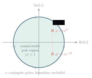
The unit circle in the $z$-plane. For a causal rational system with no hidden unstable pole-zero cancellations, BIBO stability requires every pole, including each member of a complex-conjugate pair, to lie strictly inside the unit circle.

Note

Example — Difference equation, frequency response, and stability

For the initially relaxed system

$$y[n]-\tfrac12y[n-1]=x[n],$$

the bilateral Z-transform gives

$$H(z)=\frac{Y(z)}{X(z)}=\frac{1}{1-\tfrac12z^{-1}}.$$

The causal realization has ROC $\lvert z\rvert>1/2$ and impulse response

$$h[n]=(\tfrac12)^n u[n].$$

Its pole $z=1/2$ lies strictly inside the unit circle, and $\sum_n\lvert h[n]\rvert=2$, so the causal system is BIBO stable. The frequency response is

$$H(e^{\mathrm{j}\Omega})=\frac{1}{1-\tfrac12e^{-\mathrm{j}\Omega}}.$$

For $x[n]=u[n]$,

$$\begin{aligned} Y(z) &=\frac{1}{(1-z^{-1})(1-\tfrac12z^{-1})}\\ &=\frac{2}{1-z^{-1}}-\frac{1}{1-\tfrac12z^{-1}}, \end{aligned}$$

with ROC $\lvert z\rvert>1$. Therefore

$$y[n]=\left[2-(\tfrac12)^n\right]u[n].$$

The final-value theorem gives $y[\infty]=2$, agreeing with the explicit sequence. The same algebraic $H(z)$ with ROC $\lvert z\rvert<1/2$ would be anticausal and unstable because its ROC excludes the unit circle.

Laplace Transform

Bilateral and Unilateral Definitions

For signal analysis and ROC arguments, the bilateral Laplace transform is

$$X(s)=\mathcal{L}\!\left\{x(t)\right\}=\int_{-\infty}^{\infty}x(t)e^{-st}\,\mathrm{d}t, \qquad s=\sigma+\mathrm{j}\omega.$$

Its ROC is the set of values of $s$ for which the integral converges. The factor $e^{-\sigma t}$ permits a wider class of signals than the ordinary Fourier transform.

For causal differential equations with initial conditions, use

$$X_u(s)=\mathcal{L}_u\{x(t)\} =\int_{0^-}^{\infty}x(t)e^{-st}\,\mathrm{d}t.$$

The lower limit $0^-$ includes any event at the origin and allows initial conditions to enter the transformed differential equation.

Tip

Exam Focus — Do not mix the two Laplace conventions

Bilateral transforms carry ROC and two-sided-signal information. Unilateral transforms naturally incorporate initial conditions. Their formulas must not be mixed. For the right-sided signals in the table, the two definitions produce the same algebraic expressions, but they answer different questions.

For a rational bilateral transform, the ROC is a vertical half-plane or strip that contains no pole. A right-sided signal has an ROC to the right of its rightmost pole, a left-sided signal has an ROC to the left of its leftmost pole, and a two-sided signal has a strip between pole locations. Thus, as in the Z-domain, the algebraic expression and ROC must be specified together.

Common Pairs

$x(t)$	$X(s)$	Bilateral ROC
$\delta(t)$	$1$	All $s$
$u(t)$	$\dfrac{1}{s}$	$\operatorname{Re}(s)>0$
$e^{-at}u(t)$	$\dfrac{1}{s+a}$	$\operatorname{Re}(s)>-a$
$-e^{-at}u(-t)$	$\dfrac{1}{s+a}$	$\operatorname{Re}(s)<-a$
$\sin(\omega_0t)u(t)$	$\dfrac{\omega_0}{s^2+\omega_0^2}$	$\operatorname{Re}(s)>0$
$\cos(\omega_0t)u(t)$	$\dfrac{s}{s^2+\omega_0^2}$	$\operatorname{Re}(s)>0$
$t^n u(t)$, $n=0,1,2,\ldots$	$\dfrac{n!}{s^{n+1}}$	$\operatorname{Re}(s)>0$

Common bilateral Laplace-transform pairs.

For example,

$$\int_0^\infty e^{-at}e^{-st}\,\mathrm{d}t =\frac{1}{s+a} \quad\text{only when}\quad \operatorname{Re}(s)>-a.$$

The left-sided exponential in the next row has the same algebraic expression but converges in the opposite half-plane. Its ROC, not the fraction alone, selects the inverse transform.

Properties and Value Theorems

For bilateral transforms, provided the indicated integrals and boundary terms exist, the core properties are:

Property	Time-domain operation	Transform-domain result
Linearity	$\alpha x(t)+\beta y(t)$	$\alpha X(s)+\beta Y(s)$
Time shift	$x(t-t_0)$	$e^{-st_0}X(s)$
Exponential shift	$e^{at}x(t)$	$X(s-a)$
Time differentiation	$\dfrac{\mathrm{d}x(t)}{\mathrm{d}t}$	$sX(s)$
Multiplication by $t$	$t x(t)$	$-\dfrac{\mathrm{d}X(s)}{\mathrm{d}s}$
Convolution	$x_1(t)*x_2(t)$	$X_1(s)X_2(s)$

Core bilateral Laplace-transform properties.

The differentiation, integration, and value-theorem formulas below instead use the unilateral transform and retain the initial conditions.

Property	Result
Differentiation	$\mathcal{L}_u\{x'(t)\}=sX_u(s)-x(0^-)$
Integration	$\displaystyle
\mathcal{L}_u!\left{\int_0^t x(\tau),\mathrm{d}\tau\right}
=\frac{X_u(s)}{s}$
Causal convolution	$x_1(t)*x_2(t)\leftrightarrow X_1(s)X_2(s)$
Initial value	$\displaystyle x(0^+)=\lim_{s\to\infty}sX_u(s)$
Final value	$\displaystyle
\lim_{t\to\infty}x(t)=\lim_{s\to0}sX_u(s)$, when its pole condition holds

Key unilateral Laplace-transform properties.

For an $m$th derivative, the complete initial-condition formula is

$$\mathcal{L}_u\{x^{(m)}(t)\} =s^mX_u(s)-\sum_{k=0}^{m-1}s^{m-1-k}x^{(k)}(0^-).$$

Note

Key Point — Qualifications for the Laplace value theorems

The initial-value theorem assumes that $x(t)$ has no impulse at $t=0$. The final-value theorem is valid only when every pole of $sX_u(s)$ lies strictly in the open left half-plane. Equivalently, $X_u(s)$ may have one simple pole at the origin, while all its other poles lie strictly in the open left half-plane. Under these conditions the time-domain final value exists.

Relation to the Fourier Transform and Stability

The Fourier transform is the bilateral Laplace transform evaluated on the imaginary axis:

Caution

Key Formula — Fourier–Laplace relation

$$X_F(\omega)=X_L(s)\big|_{s=\mathrm{j}\omega},$$

provided that the bilateral Laplace ROC contains the complete $\mathrm{j}\omega$-axis.

Substitution of $s=\mathrm{j}\omega$ is therefore not sufficient by itself; the ROC qualification is essential. For a causal rational continuous-time LTI system with no hidden unstable cancellations, BIBO stability requires every pole to lie strictly in the open left half-plane.

More explicitly, for the reduced rational function

$$H(s)=K\frac{\prod_k(s-z_k)}{\prod_m(s-p_m)},$$

the general BIBO condition is that the ROC of $H(s)$ contain the complete $\mathrm{j}\omega$-axis. A causal rational $H(s)$ has an ROC to the right of its rightmost pole, so causality and BIBO stability together require $\operatorname{Re}(p_m)<0$ for every pole. A pole on the imaginary axis is excluded from strict BIBO stability. Zeros do not determine stability, and an unstable pole-zero cancellation can conceal an internally unstable mode.

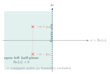
The $s$-plane for a causal rational system. BIBO-stable poles lie strictly in the open left half-plane. The Fourier transform is obtained from the bilateral Laplace transform only when its ROC contains the complete $\mathrm{j}\omega$-axis.

Note

Example — Unilateral Laplace transform with an initial condition

Solve

$$y'(t)+2y(t)=u(t), \qquad y(0^-)=1.$$

The unilateral transform gives

$$sY(s)-1+2Y(s)=\frac{1}{s},$$

and hence

$$\begin{aligned} Y(s)&=\frac{s+1}{s(s+2)} =\frac{1/2}{s}+\frac{1/2}{s+2},\\ y(t)&=\frac12+\frac12e^{-2t},\qquad t\geq0. \end{aligned}$$

The initial-value theorem gives $y(0^+)=1$. Since $sY(s)$ has only the pole $s=-2$, the final-value theorem is valid and gives $y(\infty)=1/2$. The zero-state transfer function $H(s)=1/(s+2)$ is causal and BIBO stable because its pole lies in the open left half-plane.

Fourier, Laplace, and Z Transform Comparison

Tip

Exam Focus — NTC 2079: exact 10-mark composite

This section is the exact NTC 2079 composite $[4+4+2=10]$. Reproduce all three limbs together: (a) distinguish FT, LT, and ZT using the table below $[4]$; (b) derive the Fourier transform of the impulse $[4]$; and (c) state the properties of convolution $[2]$.

Feature	Fourier transform	Laplace transform	Z-transform
Signal domain	Continuous time	Continuous time	Discrete time
Variable	$\mathrm{j}\omega$ (imaginary axis only)	$s=\sigma+\mathrm{j}\omega$ (whole plane)	$z=re^{\mathrm{j}\Omega}$ (whole plane)
Definition	$\displaystyle\int_{-\infty}^{\infty}x(t)e^{-\mathrm{j}\omega t}\,\mathrm{d}t$	$\displaystyle\int_{-\infty}^{\infty}x(t)e^{-st}\,\mathrm{d}t$	$\displaystyle\sum_{n=-\infty}^{\infty}x[n]z^{-n}$
Exists for	$L^1$ is sufficient for the ordinary FT; distributions extend it further	Wider class through $\sigma$ and the ROC	Wider class through radius $r$ and the ROC
Initial conditions	Not handled	Handled naturally	Handled by the unilateral Z-transform
Main use	Spectrum, filters, and communication	Transients, circuits, control, and stability	Digital filters, DSP, and discrete control
Stability test for causal rational systems	Not a pole-plane test	Poles strictly in the open left half-plane	Poles strictly inside the unit circle
Special-case relation	Bilateral LT on $s=\mathrm{j}\omega$	Generalizes the continuous-time FT	DTFT is ZT on $z=e^{\mathrm{j}\Omega}$

Complete comparison of the Fourier, Laplace, and Z transforms.

The Fourier Family at a Glance

The four Fourier representations are organized by whether time is continuous or discrete and whether the signal is periodic or aperiodic.

Signal	Representation	Spectrum
Continuous-time, periodic	Fourier series (FS)	Discrete lines, aperiodic
Continuous-time, aperiodic	Fourier transform (FT)	Continuous, aperiodic
Discrete-time, aperiodic	DTFT	Continuous, $2\pi$-periodic
Discrete-time, periodic or finite	DFT	Discrete, periodic

The Fourier family of signal representations.

Laplace generalizes the FT and Z generalizes the DTFT by adding a real convergence factor, respectively $\sigma$ and radius $r$. This addition provides an ROC and enables transient or initial-condition analysis.

Note

Key Point — Special-case relations

Subject to the stated convergence conditions,

$$\begin{aligned} X_F(\omega)&=X_L(s)\big|_{s=\mathrm{j}\omega},\\ X_{\mathrm{DTFT}}(e^{\mathrm{j}\Omega}) &=X_Z(z)\big|_{z=e^{\mathrm{j}\Omega}},\\ X[k]&=X_{\mathrm{DTFT}}(e^{\mathrm{j}\Omega}) \big|_{\Omega=2\pi k/N} \quad\text{for an $N$-sample record}. \end{aligned}$$

The first relation requires the bilateral Laplace ROC to contain the complete imaginary axis; the second requires the Z-transform ROC to contain the unit circle.

Fourier Transform of the Impulse

Using the sifting property,

Caution

Key Formula — Transform of a unit impulse

$$\begin{aligned} \mathcal{F}\!\left\{\delta(t)\right\} &=\int_{-\infty}^{\infty}\delta(t)e^{-\mathrm{j}\omega t}\,\mathrm{d}t \\ &=e^{-\mathrm{j}\omega\cdot0}=1. \end{aligned}$$

Thus $\delta(t)\leftrightarrow1$: the impulse contains all frequencies with equal magnitude. Under the same angular-frequency convention, Fourier duality supplies the companion pair

$$1\longleftrightarrow2\pi\delta(\omega).$$

Properties of Convolution

For

$$y(t)=x(t)*h(t) =\int_{-\infty}^{\infty}x(\tau)h(t-\tau)\,\mathrm{d}\tau,$$

the properties requested in the NTC 2079 question are:

1. Commutative: $x*h=h*x$.

2. Associative: $(x*h_1)*h_2=x*(h_1*h_2)$.

3. Distributive: $x*(h_1+h_2)=x*h_1+x*h_2$.

4. Identity and shift: $x*\delta(t)=x(t)$ and $x*\delta(t-t_0)=x(t-t_0)$.

5. Transform relation: $x*h\leftrightarrow X(\omega)H(\omega)$; time-domain convolution becomes frequency-domain multiplication.

6. Width and area: for finite-duration signals, the support endpoints add, so the nominal support duration of $x*h$ is the sum of the two support durations unless cancellation shortens it. When the required integrals exist,

$$\int_{-\infty}^{\infty}(x*h)(t)\,\mathrm{d}t =\left(\int_{-\infty}^{\infty}x(t)\,\mathrm{d}t\right) \left(\int_{-\infty}^{\infty}h(t)\,\mathrm{d}t\right).$$

Sampling: the Continuous-to-Discrete Bridge

Sampling turns a continuous-time signal $x(t)$ into the sequence

$$x[n]=x(nT_s), \qquad T_s=\frac{1}{f_s}, \qquad \omega_s=2\pi f_s=\frac{2\pi}{T_s},$$

taken every sampling interval $T_s$. It is the operation that connects the continuous transforms (Fourier and Laplace) to the discrete transforms (DTFT, DFT, and Z).

Use the angular-frequency Fourier convention established earlier:

$$X(\omega)=\int_{-\infty}^{\infty}x(t)e^{-\mathrm{j}\omega t}\,\mathrm{d}t, \qquad x(t)=\frac{1}{2\pi}\int_{-\infty}^{\infty} X(\omega)e^{\mathrm{j}\omega t}\,\mathrm{d}\omega.$$

For ideal impulse sampling, define the Dirac comb

$$p_{T_s}(t)=\sum_{n=-\infty}^{\infty}\delta(t-nT_s).$$

Its Fourier transform is another impulse train:

$$P_{T_s}(\omega) =\frac{2\pi}{T_s}\sum_{k=-\infty}^{\infty} \delta(\omega-k\omega_s) =\omega_s\sum_{k=-\infty}^{\infty} \delta(\omega-k\omega_s).$$

Multiplication in time becomes convolution in frequency, so

$$\begin{aligned} x_s(t) &=x(t)p_{T_s}(t) =\sum_{n=-\infty}^{\infty}x(nT_s)\delta(t-nT_s),\\ X_s(\omega) &=\frac{1}{2\pi}\bigl[X*P_{T_s}\bigr](\omega)\\ &=\frac{1}{T_s}\sum_{k=-\infty}^{\infty} X(\omega-k\omega_s). \end{aligned}$$

Caution

Key Formula — Exact spectrum-replication scale

$$\boxed{X_s(\omega)=\frac{1}{T_s} \sum_{k=-\infty}^{\infty}X(\omega-k\omega_s)}.$$

Every replica is centred at $k\omega_s$ and scaled by $1/T_s$. Under the hertz convention $X(f)=\int x(t)e^{-\mathrm{j}2\pi ft}\,\mathrm{d}t$, the equivalent formula is

$$X_s(f)=\frac{1}{T_s}\sum_{k=-\infty}^{\infty}X(f-kf_s).$$

Since the Fourier transform of $x_s(t)$ can also be taken directly,

$$\begin{aligned} X_s(\omega) &=\sum_{n=-\infty}^{\infty}x[n]e^{-\mathrm{j}(\omega T_s)n} =X_d(e^{\mathrm{j}\Omega})\big|_{\Omega=\omega T_s},\\ X_d(e^{\mathrm{j}\Omega}) &=\frac{1}{T_s}\sum_{k=-\infty}^{\infty} X\!\left(\frac{\Omega-2\pi k}{T_s}\right). \end{aligned}$$

This is the explicit bridge from the analog Fourier transform to the $2\pi$-periodic DTFT. Analog frequencies separated by integer multiples of $f_s$ map to the same discrete frequency modulo $2\pi$.

Sampling Theorem and Nyquist Terminology

Note

Law — Sampling theorem

A signal band-limited to a maximum frequency $f_m$ can be recovered uniquely from its samples only if

$$\boxed{f_s\geq2f_m}.$$

The theoretical minimum $2f_m$ is the Nyquist rate. The frequency $f_s/2$ is the Nyquist frequency, also called the folding frequency. These two terms are related but are not interchangeable.

Equality is the ideal mathematical boundary. Practical anti-alias filters need a finite transition band, so a realizable system normally samples above $2f_m$ and leaves a guard band.

Spectrum Replication, Aliasing, and Filtering

Ideal sampling places a scaled copy of $X(f)$ at every integer multiple of $f_s$. If $f_s\geq2f_m$, adjacent copies remain separate and the baseband copy is intact. If $f_s<2f_m$, neighboring copies overlap: components above the folding frequency map to lower apparent frequencies. This irreversible spectral corruption is aliasing.

An analog anti-aliasing low-pass filter must therefore band-limit $x(t)$ to below $f_s/2$ before the sampler. Filtering after sampling cannot separate spectral components that have already folded onto one another.

For sampled complex sinusoids,

$$e^{\mathrm{j}2\pi(f+kf_s)nT_s}=e^{\mathrm{j}2\pi f nT_s}, \qquad k\in\mathbb{Z}.$$

A real sinusoid at $f_{\mathrm{in}}$ therefore appears in the principal Nyquist interval at

Caution

Key Formula — Folded alias frequency

$$f_a=\min_{k\in\mathbb{Z}}\lvert f_{\mathrm{in}}-kf_s\rvert, \qquad 0\leq f_a\leq\frac{f_s}{2}.$$

No digital filter can undo this identification after the samples have been formed. A realizable design uses an analog anti-alias filter, a guard band, and often oversampling.

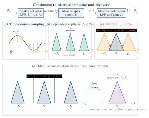
Ideal sampling and reconstruction. An analog anti-alias filter band-limits the input before time-domain sampling. Adequate sampling keeps the spectral replicas separate; undersampling makes them overlap and alias. An ideal reconstruction low-pass filter retains the baseband replica and rejects the images.

Note

Example — Sampling-rate check and folded alias

A 7 kHz sinusoid is sampled at $f_s=10\,kHz$. Its theoretical Nyquist rate is $2f_m=14\,kHz$, so the chosen sampler violates the theorem. The observed alias is

$$f_a=\lvert7-1(10)\rvert=3\,kHz.$$

Indeed,

$$\cos\!\left(2\pi\frac{7}{10}n\right) =\cos\!\left(2\pi n-2\pi\frac{3}{10}n\right) =\cos\!\left(2\pi\frac{3}{10}n\right).$$

The 7 kHz and 3 kHz sinusoids therefore produce identical sample values. To preserve the 7 kHz component, raise $f_s$ above 14 kHz with a practical guard band. If it is unwanted, an analog filter below the 5 kHz folding frequency must remove it before the 10 kHz sampler.

Ideal and Practical Reconstruction

Assume $X(\omega)=0$ for $\lvert\omega\rvert>\omega_m$ and $\omega_s>2\omega_m$. An ideal reconstruction low-pass filter rejects the images and retains the baseband copy. Since ideal sampling scales that copy by $1/T_s$, the reconstruction passband must have gain $T_s$:

$$H_r(\omega)= \begin{cases} T_s, & \lvert\omega\rvert\leq\omega_c,\\ 0, & \lvert\omega\rvert>\omega_c, \end{cases} \qquad \omega_m\leq\omega_c\leq\omega_s-\omega_m.$$

A common ideal choice is $\omega_c=\omega_s/2$. In the time domain, this brick-wall operation is sinc interpolation:

Caution

Key Formula — Ideal band-limited interpolation

$$x(t)=\sum_{n=-\infty}^{\infty}x[n] \operatorname{sinc}\!\left(\frac{t-nT_s}{T_s}\right), \qquad \operatorname{sinc}(v)=\frac{\sin(\pi v)}{\pi v}.$$

Each sample weights a shifted sinc pulse whose zeros occur at all the other sampling instants. This exact result assumes ideal band limitation and an ideal reconstruction filter. The ideal sinc is noncausal and infinite in duration, while the ideal brick-wall filter is unrealizable. Practical systems instead use a sample-and-hold or zero-order hold followed by an analog reconstruction (anti-imaging or smoothing) filter. Oversampling provides transition width, and practical designs may compensate the hold’s sinc-shaped passband droop.

Note

Key Point — Where the full conversion chain is treated

Within these notes, sample-and-hold circuits, quantization, and companding are developed in Subject 05 under Analog-to-Digital Conversion. The full sampling, quantization, encoding, transmission, and decoding chain is treated there under PCM and ADPCM. These local topic names replace the source web links and remain usable in the printed compendium.

Quick Review

• Fourier series represents periodic signals; the Fourier transform represents aperiodic signals.

• Convolution in time becomes multiplication in frequency.

• The unit impulse has the sifting property and $\mathcal{F}\!\left\{\delta(t)\right\}=1$.

• The Hilbert transform supplies a $90^\circ$ phase shift and forms the analytic signal; its detailed properties and SSB application are covered in Section 4.5.

• The Z-transform is the principal tool for discrete-time LTI systems and digital filters; its ROC is essential.

• The four Fourier representations are FS (continuous-time periodic), FT (continuous-time aperiodic), DTFT (discrete-time aperiodic with a $2\pi$-periodic spectrum), and DFT (discrete-time finite with a discrete, periodic spectrum).

• The sampling condition is $f_s\geq2f_m$. Below the Nyquist rate, aliasing folds high frequencies downward; an anti-alias filter must act before sampling.

• Parseval’s theorem preserves energy between time and frequency. Under the angular-frequency convention, Fourier duality pairs $\delta(t)\leftrightarrow1$ with $1\leftrightarrow2\pi\delta(\omega)$.

• The FT–LT–ZT comparison, the impulse transform, and the convolution properties form the exact NTC 2079 composite question and should be reproduced together.