Bode Plot Analysis

Definition, Logarithmic Conventions and Factorisation

A Bode plot consists of (i) magnitude $20\log_{10}|H(j\omega)|$ in decibels and (ii) phase $\angle H(j\omega)$ in degrees, both plotted against logarithmic frequency. The log axis compresses a wide range and converts multiplication of transfer- function factors into addition of their magnitude and phase contributions.

For an amplitude ratio,

$$M(\omega)=20\log_{10}|H(j\omega)|\ \text{dB},$$

whereas a power ratio uses

$$G_P=10\log_{10}\left(\frac{P_o}{P_i}\right)\ \text{dB}.$$

Thus $|H|=1$ is $0$ dB, $|H|=10$ is $20$ dB, $|H|=0.1$ is $-20$ dB, and an amplitude factor $1/\sqrt{2}$ is $-3.01$ dB. A decade is a frequency ratio of $10:1$ and an octave a ratio of $2:1$; $20$ dB/decade is approximately $6.02$ dB/octave.

Angular and ordinary frequency are related by

$$\omega=2\pi f.$$

A numerical corner must carry the convention used. A logarithmic axis cannot contain $\omega=0$; DC behavior is inferred from the limiting transfer function.

Normalised pole-zero form

A real-rational transfer function can be arranged as

$$\begin{aligned} H(s)={}&K\,s^{q} \frac{\displaystyle \prod_i\left(1+\frac{s}{\omega_{zi}}\right)^{m_i} \prod_k\left[1+2\zeta_{zk}\frac{s}{\omega_{nzk}} +\left(\frac{s}{\omega_{nzk}}\right)^2\right]^{r_k}} {\displaystyle \prod_j\left(1+\frac{s}{\omega_{pj}}\right)^{n_j} \prod_\ell\left[1+2\zeta_{p\ell}\frac{s}{\omega_{np\ell}} +\left(\frac{s}{\omega_{np\ell}}\right)^2\right]^{t_\ell}}. \end{aligned}$$

Here $q>0$ denotes $q$ more zeros than poles at the origin; $q<0$ denotes $|q|$ more poles. Exponents represent repeated factors. Constants extracted while normalising factors must be absorbed into $K$. This avoids the common error of treating $(s+a)$ as $(1+s/a)$ without multiplying the gain by $a$.

For example,

$$\frac{s+10}{s(s+100)} =\frac{10(1+s/10)}{100s(1+s/100)} =0.1\frac{1+s/10}{s(1+s/100)}.$$

Note

Key Point — Corner and Cutoff Are Not Always Synonyms

A corner or break frequency belongs to a normalised pole/zero factor and marks an asymptotic slope change. A cutoff is a specified passband edge. They coincide at the $-3.01$ dB point of an isolated first-order section, but need not coincide in higher-order, interacting or rippled responses.

Standard Bode Factors

Constant and origin factors

For a real constant $K$,

$$M_K=20\log_{10}|K|, \qquad \phi_K= \begin{cases} 0^\circ,&K>0,\\ \pm180^\circ,&K<0. \end{cases}$$

The $\pm180^\circ$ representation is selected to keep the unwrapped phase continuous.

A zero at the origin, $H=s$, gives

$$M=20\log_{10}\omega, \qquad \phi=+90^\circ,$$

and therefore a $+20$ dB/decade line through $0$ dB at $\omega=1\,\text{rad/s}$. A pole at the origin, $H=1/s$, gives the negative of both contributions. For $s^q$, slope and phase are respectively $20q$ dB/decade and $90q^\circ$.

First-order real zero and pole

Let $r=\omega/\omega_c$. A left-half-plane zero is

$$H_z(j\omega)=1+jr,$$

with exact contribution

$$M_z=10\log_{10}(1+r^2),\qquad \phi_z=\tan^{-1}r.$$

Its low-frequency magnitude asymptote is $0$ dB; above $\omega_c$ its slope is $+20$ dB/decade and phase tends to $+90^\circ$.

A pole is the reciprocal:

$$H_p(j\omega)=\frac{1}{1+jr},$$

so

$$M_p=-10\log_{10}(1+r^2),\qquad \phi_p=-\tan^{-1}r.$$

At $r=1$, a zero contributes $+3.01$ dB and $+45^\circ$; a pole contributes $-3.01$ dB and $-45^\circ$. A factor repeated $n$ times multiplies its dB, phase and eventual slope by $n$.

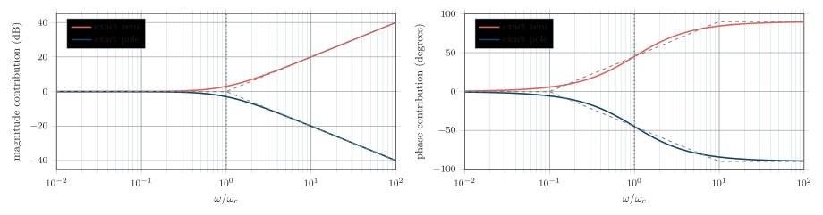
Native exact and straight-line first-order contributions. Dashed curves are the asymptotic magnitude and one-decade phase approximations.

Complex second-order factors

A standard left-half-plane pole pair is

$$H_{2p}(s)=\frac{1}{1+2\zeta(s/\omega_n)+(s/\omega_n)^2}.$$

With $r=\omega/\omega_n$,

$$\begin{aligned} M_{2p}&=-10\log_{10}\left[(1-r^2)^2+(2\zeta r)^2\right], \\ \phi_{2p}&=-\operatorname{atan2}(2\zeta r,1-r^2), \end{aligned}$$

where phase is unwrapped continuously from $0^\circ$ toward $-180^\circ$. The high-frequency slope is $-40$ dB/decade. At $\omega_n$,

$$M_{2p}(\omega_n)=-20\log_{10}(2\zeta).$$

Thus an underdamped pair can peak; for $\zeta=1/\sqrt{2}$ the value is $-3.01$ dB, and for $\zeta=1$ it is $-6.02$ dB. A second-order zero has the opposite magnitude and phase contributions. Repeated pairs multiply the contributions by their multiplicity.

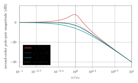
Native second-order pole-pair magnitude. Damping determines the near-resonance correction even though all curves approach the same asymptotes.

Note

Key Point — Magnitude Does Not Determine Phase Uniquely

A right-half-plane zero $1-s/\omega_z$ has the same magnitude as the left-half-plane zero $1+s/\omega_z$ but contributes phase lag rather than lead. A pure delay $e^{-sT}$ has $0$ dB magnitude and phase $-\omega T$ radians. Therefore a magnitude-only sketch cannot reveal non-minimum-phase zeros or delay; use the actual factor signs and phase model.

Straight-Line Construction and Exact Corrections

Construction algorithm

For hand construction:

1. Factor and normalise $H(s)$ as in the equation; include constants extracted from every $(s+a)$ factor in $K$.

2. List all origin factors, real corners, multiplicities, second-order natural frequencies and damping ratios in ascending frequency.

3. Choose a convenient reference frequency below the first finite corner. Evaluate the constant/origin magnitude there and determine the initial slope.

4. Continue the magnitude line through each corner, changing cumulative slope by $+20m$ dB/decade for $m$ real zeros, $-20n$ for $n$ real poles, and $\pm40$ per second-order pair.

5. Add phase algebraically. For a first-order LHP factor, use the exact $\pm\tan^{-1}(\omega/\omega_c)$ or the straight-line transition from one decade below to one decade above its corner.

6. Apply exact corner/resonance corrections where accuracy matters, then mark cutoffs, bandwidth or loop-gain crossovers from the resulting curves.

The straight-line phase approximation for one LHP zero is

$$\phi_z\simeq \begin{cases} 0^\circ,&\omega\leq0.1\omega_z,\\ 45^\circ\left[1+\log_{10}(\omega/\omega_z)\right], &0.1\omega_z<\omega<10\omega_z,\\ 90^\circ,&\omega\geq10\omega_z, \end{cases}$$

with the sign reversed for a pole. Overlapping transitions must be added; phase does not jump instantaneously at a corner.

Exact versus asymptotic values

$r=\omega/\omega_c$	$0.1$	$0.5$	$1$	$2$	$10$
Zero correction	$+0.043$ dB	$+0.969$ dB	$+3.010$ dB	$+0.969$ dB	$+0.043$ dB
Pole correction	$-0.043$ dB	$-0.969$ dB	$-3.010$ dB	$-0.969$ dB	$-0.043$ dB
Exact phase magnitude	$5.71^\circ$	$26.57^\circ$	$45^\circ$	$63.43^\circ$	$84.29^\circ$

Exact first-order correction relative to its magnitude asymptote.

For a zero, the exact curve lies above both magnitude asymptotes; for a pole it lies below. Corrections add in dB and multiply by factor repetition. Closely spaced corners interact through addition of their exact contributions, so the overall cutoff cannot be found by correcting each section in isolation and then simply choosing one corner.

Common response shapes

Response	Magnitude behavior	Typical phase trend
Low-pass	Flat low-frequency band, then rolls off above $f_H$	$0^\circ$ toward $-90^\circ$ per first-order pole
High-pass	Rises below $f_L$, then becomes flat	$+90^\circ$ toward $0^\circ$ for one first-order section
Band-pass	Passes $f_L<f<f_H$; $BW=f_H-f_L$	Lead below centre and lag above centre
Band-stop/notch	Passes outside a rejected band, often with a zero at $f_0$	Rapid phase transition around the rejection frequency

Standard transfer-function response shapes.

These names describe the chosen input-to-output transfer function. The same series or parallel resonator can realise different responses depending on where it is inserted and where output is measured.

Fully Worked Bode Construction

Note

Example — Three-Corner Magnitude and Phase Plot

Construct the Bode plot of

$$G(s)=\frac{100(1+s/10)}{s(1+s/100)(1+s/1000)}.$$

All finite corner frequencies are in rad/s. The factors are:

• $K=100$, contributing $40$ dB and $0^\circ$;

• one pole at the origin, contributing an initial $-20$ dB/decade slope and $-90^\circ$;

• one zero at $10\,\text{rad/s}$;

• one pole at $100\,\text{rad/s}$; and

• one pole at $1000\,\text{rad/s}$.

At $\omega=1\,\text{rad/s}$, well below the first finite corner, $|G|\simeq100$, or $40$ dB. The cumulative slope walk is

Frequency interval	Slope	Reason
$\omega<10$	$-20$ dB/dec	pole at origin
$10<\omega<100$	$0$	zero at 10 adds $+20$
$100<\omega<1000$	$-20$ dB/dec	pole at 100 adds $-20$
$\omega>1000$	$-40$ dB/dec	pole at 1000 adds another $-20$

Hence useful asymptotic points are

$\omega$ (rad/s)	$0.1$	$1$	$10$	$100$	$1000$	$10^4$	$10^5$
$	G	_{asym}$ (dB)	$60$	$40$	$20$	$20$	$0$

The exact magnitude and phase are

$$\begin{aligned} |G|_{dB}={}&40-20\log_{10}\omega +10\log_{10}\left[1+(\omega/10)^2\right]\nonumber\\ &-10\log_{10}\left[1+(\omega/100)^2\right] -10\log_{10}\left[1+(\omega/1000)^2\right], \\ \phi={}&-90^\circ+\tan^{-1}(\omega/10) -\tan^{-1}(\omega/100)-\tan^{-1}(\omega/1000). \end{aligned}$$

At $\omega=10,100,1000\,\text{rad/s}$, the exact magnitude/phase pairs are approximately

$$(22.97\,\text{dB},-51.3^\circ),\quad (16.99\,\text{dB},-56.4^\circ),\quad (-3.05\,\text{dB},-129.9^\circ).$$

The zero partly cancels the origin-pole phase over the middle band; the two higher poles then drive phase toward its final $-180^\circ$ value.

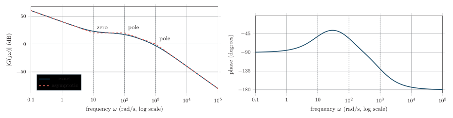
Native exact and asymptotic construction for the equation. The horizontal plotting coordinate is $\log_{10}\omega$, with physical frequencies shown on the ticks.

Loop Gain, Crossovers and Stability Margins

For the negative-feedback amplifier of the figure, closed-loop poles satisfy

$$1+L(s)=0, \qquad L(s)=A(s)\beta(s).$$

Consequently, margins are measured from the loop-gain Bode plot, not from the closed-loop response or forward gain $A$ alone.

Gain crossover and phase margin

The gain-crossover frequency $\omega_{gc}$ is any relevant frequency at which

$$|L(j\omega_{gc})|=1, \qquad L_{dB}(\omega_{gc})=0\,\text{dB}.$$

With the conventional negative-feedback sign and phase unwrapped around the relevant crossing,

Caution

Key Formula — Phase Margin

$$\boxed{PM=180^\circ+\angle L(j\omega_{gc})}.$$

Phase margin is an angle and must be reported in degrees.

It is the additional phase lag required at unity loop-gain magnitude to reach the critical $-180^\circ$ condition.

Phase crossover and gain margin

The phase-crossover frequency $\omega_{pc}$ is any relevant frequency where

$$\angle L(j\omega_{pc})=-180^\circ\pmod{360^\circ}.$$

The multiplicative and decibel gain margins are

Caution

Key Formula — Gain Margin

$$\boxed{GM=\frac{1}{|L(j\omega_{pc})|}}, \qquad \boxed{GM_{dB}=-20\log_{10}|L(j\omega_{pc})| =-L_{dB}(\omega_{pc})}.$$

Gain margin is dimensionless as a ratio or is reported in dB. State the unit.

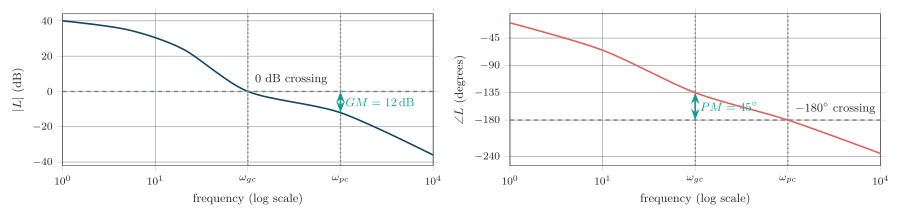
Native loop-gain Bode plots showing the correct locations of gain and phase margins.

Note

Example — Reading Margins from a Loop-Gain Plot

Suppose $\angle L=-135^\circ$ at the 0-dB crossing and $L_{dB}=-12$ dB at the $-180^\circ$ crossing. Then

$$PM=180^\circ-135^\circ=45^\circ,$$$$GM_{dB}=-(-12)=12\,\text{dB}, \qquad GM=10^{12/20}=3.98.$$

The result means that, with the loop model and relevant crossings otherwise unchanged, loop gain could increase by a factor of about four before reaching unity at the phase crossover.

Closed-loop interpretation and its limits

For the common case of a stable open-loop system, conventional negative- feedback sign and one relevant crossover:

• positive GM and PM indicate closed-loop stability;

• zero margin is marginal; negative margin indicates instability; and

• larger PM usually reduces ringing and overshoot, although reducing crossover frequency can also reduce speed and bandwidth.

Values around $45^\circ$–$60^\circ$ PM and at least $8$–$10$ dB GM are common design targets, not universal requirements.

Note

Law — Positive Margins Need the Usual Assumptions

With right-half-plane open-loop poles, multiple 0-dB or $-180^\circ$ crossings, large delay, non-minimum-phase behavior or other Nyquist-path complications, simple positive GM/PM statements may be insufficient. Apply the Nyquist criterion and inspect every relevant crossing. If no phase crossover exists, elementary gain margin may be infinite; if no gain crossover exists, phase margin may be undefined rather than automatically “very large.”

The slope near $\omega_{gc}$ also matters. A $-20$ dB/decade crossing often has useful phase margin in a minimum-phase dominant-pole loop, while a $-40$ dB/decade or steeper crossing warns that several poles are active. Slope is a diagnostic, not a substitute for evaluating phase.

Frequency Compensation

Compensation reshapes $L(s)$ so that loop gain crosses 0 dB before excessive phase lag accumulates, while retaining required low-frequency accuracy and speed.

Method	Action and trade-off
Dominant-pole compensation	Introduces a low pole so the 0-dB crossing occurs before non-dominant poles add excessive lag. Robust, but lowers bandwidth and slows settling.
Lead compensation	Places a zero below a higher pole to add positive phase near crossover. It can raise PM or crossover frequency, but may amplify high-frequency noise.
Lag compensation	Increases low-frequency loop gain relative to crossover, improving steady-state accuracy. It usually reduces speed and adds phase lag.
Miller compensation and pole splitting	An internal capacitor creates a dominant pole and moves another pole upward. Common in op-amps, but finite charging current imposes a slew-rate limit.
Pole-zero cancellation	Can reduce the effect of a known stable pole, but exact cancellation is fragile under tolerance and an unstable pole must not be hidden by nominal cancellation.

Common feedback-compensation methods.

Practical Bode-Analysis Caveats

Hand plots use linear small-signal models. A complete design must also consider:

• source and load impedances, including their frequency dependence;

• transistor, wiring and package parasitics, and frequency-dependent feedback factor $\beta(s)$;

• component tolerance, temperature, bias and model uncertainty;

• pure delays and right-half-plane zeros that add phase lag without the expected minimum-phase magnitude clue;

• clipping, slew rate, current limiting, saturation recovery and thermal effects, none of which is predicted by small-signal margins; and

• loop-gain measurement loading: an injected test signal must be small and the loop-opening method must preserve the operating point and impedances.

Use Bode construction for insight and first design, exact computation or measurement for crossover values, Nyquist analysis where topology demands it, and transient/large-signal simulation or testing for behavior outside the linear model.