Root Locus Method

Consider a continuous-time negative-feedback system with forward transfer function $G(s)$, feedback $H(s)$, and a nonnegative adjustable gain $K$. Its closed-loop transfer function and loop transfer function are

$$T(s)=\frac{K G(s)}{1+K G(s)H(s)}, \qquad L(s)=K G(s)H(s)=K L_0(s).$$

The root locus is the set of positions traced by the roots of the closed-loop characteristic equation as a real system parameter, normally $K$, varies from $0$ to $\infty$. Thus it displays the motion of every closed-loop pole directly in the $s$-plane.

The method is important because one sketch can reveal:

• the gain range for closed-loop stability;

• changes in transient speed, damping, and overshoot as $K$ changes;

• likely dominant closed-loop poles;

• damping ratio $\zeta$ and natural frequency $\omega_n$;

• the effect of adding open-loop poles or zeros; and

• whether a controller or compensator is needed to meet a design target.

Note

Key Point — Basic idea

The uncancelled open-loop poles and zeros determine the possible closed-loop pole paths. At $K=0$, the closed-loop poles start at the open-loop poles. As $K\to\infty$, each branch terminates at an open-loop zero or, when there are more poles than finite zeros, at a zero at infinity.

the figure is an exact example rather than a decorative sketch. For the nonreal branches, writing $s=x+jy$ in the angle condition gives

$$y^2=3x^2+12x+8, \qquad K=8(x+1)(x+2)(x+3),$$

with $x\ge -2+2/\sqrt3$. Therefore the plotted branches, crossing points, and arrows all correspond to $K\ge0$.

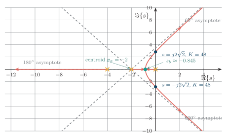
Exact root locus for $G(s)H(s)=K/(s(s+2)(s+4))$. The arrows show increasing $K$; the complex branches satisfy the angle condition and approach the three asymptotes.

Characteristic Equation and Root-Locus Conditions

The denominator of $T(s)$ gives the characteristic equation

$$\boxed{1+K G(s)H(s)=0}.$$

Equivalently,

$$K L_0(s)=-1.$$

Because $-1$ has unit magnitude and an angle equal to an odd multiple of $180^\circ$, every root-locus point must satisfy two conditions:

Caution

Key Formula — Root-locus conditions

$$\boxed{\lvert K L_0(s)\rvert=1}, \qquad \boxed{\angle L_0(s)=(2q+1)180^\circ}, \quad q=0,\pm1,\pm2,\ldots$$

Write the gain-free loop transfer function as

$$L_0(s)=\frac{N(s)}{D(s)} =\frac{\displaystyle\prod_{i=1}^{m}(s-z_i)} {\displaystyle\prod_{i=1}^{n}(s-p_i)},$$

where $z_i$ and $p_i$ are its uncancelled open-loop zeros and poles. At a candidate point $s=s_0$, the angle condition becomes

$$\boxed{ \sum_{i=1}^{m}\angle(s_0-z_i) -\sum_{i=1}^{n}\angle(s_0-p_i) =(2q+1)180^\circ}.$$

Only after this angle test is satisfied may the magnitude condition be used to find the corresponding nonnegative gain:

$$\boxed{ K=\frac{1}{\lvert L_0(s_0)\rvert} =\frac{\displaystyle\prod_{i=1}^{n}\lvert s_0-p_i\rvert} {\displaystyle\prod_{i=1}^{m}\lvert s_0-z_i\rvert}}.$$

Tip

Exam Focus — Use both conditions

The magnitude calculation alone does not prove that a selected point lies on the root locus. First check the odd-$180^\circ$ angle condition; then compute $K$ from the distance ratio.

Ten Construction Rules

Assume a real-coefficient, proper loop transfer function with $n\ge m$ and $K\ge0$. The following rules convert the two exact locus conditions into a systematic sketch.

Number of branches

The closed-loop characteristic equation is

$$F(s,K)=D(s)+K N(s)=0.$$

Its degree is $n$, so it has $n$ roots when multiplicity is counted. Hence

$$\boxed{\text{number of root-locus branches}=n.}$$

Starting and ending points

At $K=0$, $F(s,0)=D(s)$, so branches start at the $n$ open-loop poles. For large $K$, $N(s)$ must approach zero for a finite root, so $m$ branches end at the finite open-loop zeros. The remaining $n-m$ branches end at infinity:

$$\boxed{n\text{ starts at poles},\quad m\text{ ends at finite zeros},\quad n-m\text{ ends at infinity}.}$$

Repeated poles or zeros receive the corresponding number of branches.

Symmetry

Since $F(s,K)$ has real coefficients for real $K$, every nonreal root occurs with its complex conjugate. The root locus is therefore symmetric about the real axis. It is enough to construct one half and reflect it.

Real-axis segments

Take a test point on the real axis that is not itself a pole or zero. A real pole or zero to its left contributes an angle of $0^\circ$, while one to its right contributes $180^\circ$. Nonreal conjugate singularities contribute angles whose sum is an even multiple of $180^\circ$. Therefore:

Note

Law — Real-axis odd-count rule

A real-axis point belongs to the $K\ge0$ root locus if and only if the number of real open-loop poles and zeros strictly to its right is odd.

Apply the count separately on every interval divided by a real pole or zero.

Asymptotes and centroid

If $n>m$, let $r=n-m$. Far from all finite poles and zeros, $L_0(s)\sim s^{m-n}=s^{-r}$. Applying the angle condition to $s=R e^{j\theta}$ as $R\to\infty$ yields the $r$ asymptote directions

$$\boxed{ \theta_q=\frac{(2q+1)180^\circ}{n-m}, \qquad q=0,1,\ldots,n-m-1.}$$

Matching the first-order terms of the pole and zero products, or equivalently using the sum of roots, locates the common real-axis intercept:

$$\boxed{ \sigma_a=\frac{\displaystyle\sum_{i=1}^{n}p_i -\displaystyle\sum_{i=1}^{m}z_i}{n-m}.}$$

The pole and zero locations in this expression are algebraic, so an LHP pole such as $-4$ contributes $-4$; dropping that sign reverses the centroid.

Breakaway and break-in points

On the locus, solve the characteristic equation for gain:

$$K(s)=-\frac{D(s)}{N(s)}.$$

At a multiple closed-loop root, both $F(s,K)=0$ and $\partial F/\partial s=0$. Away from an open-loop zero this is equivalent to

$$\boxed{\frac{dK(s)}{ds}=0.}$$

A real stationary point where two branches leave the real axis is a breakaway; one where they enter is a break-in. The derivative equation produces candidates only. A candidate is retained only if it lies on a valid real-axis segment, satisfies the angle condition, and gives $K\ge0$.

Tip

Exam Focus — Reject invalid derivative roots

Never plot every solution of $dK/ds=0$. Mark the real-axis locus first and substitute each candidate into $K(s)$; a point on an even-count interval or a point giving negative gain is not on the conventional root locus.

Angle of departure from a complex pole

Let $p_k$ be a complex open-loop pole. Apply the angle condition at a point infinitesimally displaced from $p_k$ and isolate the angle of that displacement. The departure angle, measured from the positive real axis into the branch, is

$$\boxed{ \phi_d=180^\circ +\sum_{i=1}^{m}\angle(p_k-z_i) -\sum_{\substack{i=1\\i\ne k}}^{n}\angle(p_k-p_i) \pmod{360^\circ}.}$$

The conjugate pole has the reflected departure angle.

Angle of arrival at a complex zero

Similarly, at a complex zero $z_k$, isolate the angle of the local ray from the zero into the nearby locus. The arrival-angle formula is

$$\boxed{ \phi_a=180^\circ -\sum_{\substack{i=1\\i\ne k}}^{m}\angle(z_k-z_i) +\sum_{i=1}^{n}\angle(z_k-p_i) \pmod{360^\circ}.}$$

All vector angles must be evaluated in the correct quadrant; an $\operatorname{atan2}$ calculation is safer than an unqualified inverse tangent.

Imaginary-axis crossing

Insert the gain-dependent characteristic polynomial into a Routh array. A crossing occurs at the gain for which a first-column boundary is reached, normally producing an all-zero row. The row above supplies an auxiliary polynomial $A(s)$; its imaginary roots give the crossing frequency. Direct substitution $s=j\omega$ and separation of real and imaginary parts is a useful independent check.

Gain at any locus point

For any point already verified by the angle condition, use the distance form of the magnitude condition:

$$\boxed{ K=\frac{\displaystyle\prod_i\lvert s-p_i\rvert} {\displaystyle\prod_i\lvert s-z_i\rvert}.}$$

This labels the locus with gain and determines the direction of increasing $K$ from the start points toward finite zeros or infinity.

Stability and Gain Range

A finite-dimensional continuous-time closed loop is asymptotically stable, and its proper rational transfer function is BIBO stable, when every uncancelled closed-loop pole lies strictly in the open left half-plane (LHP). Root locus exposes this condition for every plotted value of $K$.

Closed-loop pole location at a given $K$	Interpretation
All branches strictly in the LHP	Stable for that gain
One or more branches in the RHP	Unstable for that gain
Simple conjugate pair on the imaginary axis, all others in the LHP	Stability boundary; sustained zero-input oscillation, but not BIBO stable
Repeated imaginary-axis pole	Unstable because the natural response grows polynomially

Reading closed-loop stability from a root locus

To obtain an exact stable-gain range:

1. Form $1+K L_0(s)=0$ and expand its characteristic polynomial.

2. Construct the Routh array with the leading coefficient normalized positive.

3. Require every first-column element to be strictly positive.

4. Solve the resulting simultaneous inequalities in $K$.

5. Check that every endpoint agrees with the root-locus crossing or termination shown in the $s$-plane.

Routh–Hurwitz Support

For

$$a_n s^n+a_{n-1}s^{n-1}+\cdots+a_1s+a_0=0,$$

the first two rows of the Routh array are filled alternately from the coefficients, and subsequent entries are formed from the preceding two rows. For a fourth-order polynomial,

$$\begin{array}{c|ccc} s^4 & a_4 & a_2 & a_0 \\ s^3 & a_3 & a_1 & 0 \\ s^2 & b_1 & b_2 & 0 \\ s^1 & c_1 & 0 & 0 \\ s^0 & a_0 & 0 & 0 \end{array}$$

where

$$b_1=\frac{a_3a_2-a_4a_1}{a_3}, \qquad b_2=\frac{a_3a_0-a_4(0)}{a_3}=a_0,$$

and

$$c_1=\frac{b_1a_1-a_3b_2}{b_1}.$$

Note

Law — Routh interpretation

The number of sign changes in the first column equals the number of roots in the open right half-plane. With a positive leading coefficient, no sign change and no zero first-column element means every first-column entry is positive and all roots lie in the LHP.

Two special cases must be handled rather than ignored:

• Zero first element, row not all zero: replace the zero by a small positive $\epsilon$, complete the table symbolically, and take the limit $\epsilon\to0^+$ when counting sign changes.

• Entire row zero: form the auxiliary polynomial from the row immediately above, replace the zero row by the coefficients of $dA(s)/ds$, and continue. The roots of $A(s)$ include the symmetric pair responsible for the boundary; at a root-locus crossing they give $s=\pm j\omega$.

Note

Key Point — Cross-checking a crossing

At a proposed gain $K_c$, solve the auxiliary equation for $\omega$ and also substitute $s=j\omega$ into the original characteristic equation. Both the real and imaginary parts must vanish. This catches sign errors in the Routh entries and in the stable-gain inequalities.

Transient-Response Mapping and Design Grids

For a dominant underdamped closed-loop pair, write

$$s=-\sigma\pm j\omega_d, \qquad \sigma>0.$$

The standard second-order relationships are

Caution

Key Formula — Pole location and transient response

$$\omega_n=\sqrt{\sigma^2+\omega_d^2}, \qquad \zeta=\frac{\sigma}{\omega_n},$$$$t_s\approx\frac{4}{\sigma} =\frac{4}{\zeta\omega_n}, \qquad t_p=\frac{\pi}{\omega_d},$$$$\%OS=100\exp\left( -\frac{\pi\zeta}{\sqrt{1-\zeta^2}} \right).$$

Here the settling-time formula uses the usual $2\%$ criterion and assumes a dominant second-order response. Additional poles, zeros, or large residues can make the actual response differ.

The $s$-plane design loci follow immediately:

Quantity held constant	Locus in the $s$-plane	Interpretation
Damping ratio $\zeta$	Rays from the origin with $\zeta=\cos\theta$, where $\theta$ is measured from the negative real axis	Larger $\zeta$ places the ray closer to the negative real axis and normally reduces overshoot
Natural frequency $\omega_n$	Circles $\lvert s\rvert=\omega_n$ centered at the origin	Radial distance sets $\omega_n$
Settling time $t_s$	Vertical line $\Re\{s\}=-\sigma=-4/t_s$	Poles farther left have a faster exponential envelope

Standard root-locus design-grid curves in the LHP

For example, $\zeta=0.6$ and $\omega_n=4\,\mathrm{rad/s}$ give

$$s_d=-\zeta\omega_n \pm j\omega_n\sqrt{1-\zeta^2} =-2.4\pm j3.2.$$

The point also satisfies $t_s\approx4/2.4=1.67\,\mathrm{s}$. A design-grid intersection is only a performance target; it is achievable by gain alone only when it also satisfies the plant’s root-locus angle condition.

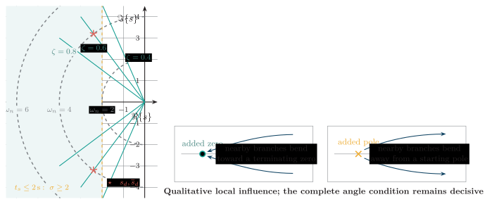
Root-locus design grid: constant-$\zeta$ rays, constant-$\omega_n$ circles, the $t_s=2\,\mathrm{s}$ boundary, a desired pole pair, and the qualitative influence of an added pole or zero.

Effect of Adding Poles and Zeros

The angle condition explains the common design heuristic that zeros attract nearby locus branches while poles repel them. This is a tendency, not an independent construction law: all poles and zeros contribute angles, so the complete compensated locus must always be reconstructed.

Adding an open-loop pole commonly bends the locus toward the right, which can reduce relative stability, slow the response, increase overshoot, or make a previous gain range unstable. Adding an open-loop zero commonly bends the locus leftward, increasing damping and speed and reducing settling time. Location matters; neither statement is universal for every plant.

Compensator	Typical root-locus addition	Main purpose
Lead	LHP zero closer to the origin than its LHP pole	Supplies positive phase and moves a feasible dominant-pole region leftward for better transient response and stability margin
Lag	LHP pole closer to the origin than its LHP zero	Raises low-frequency loop gain and improves steady-state accuracy while trying to disturb the dominant locus only slightly
PID	A pole at the origin and up to two controller zeros; a practical derivative filter may add a high-frequency pole	Combines steady-state improvement with transient-shaping freedom

Pole-zero interpretation of common compensators

Root-Locus Design Procedure

A complete gain or compensator design follows this sequence:

1. Write $L(s)=K L_0(s)=K G(s)H(s)$ and form the characteristic equation.

2. Factor $L_0(s)$ and mark every uncancelled open-loop pole and zero.

3. Construct the uncompensated root locus using all ten rules.

4. Translate overshoot, settling-time, peak-time, and frequency specifications into a desired region or desired dominant pole pair.

5. Test a desired point with the angle condition. If it lies on the locus, choose it as the dominant pair.

6. Use the magnitude condition to calculate $K$.

7. Find all remaining closed-loop poles and verify that neglected poles are sufficiently farther left and have no unexpectedly large residue.

8. If the uncompensated locus misses the desired point, calculate the angle deficiency, add a suitable lead, lag, or PID pole-zero pattern, reconstruct the locus, and verify both transient and steady-state requirements.

If percent overshoot is specified, put $M_p=(\%OS)/100$. Inverting the overshoot relation gives

$$\boxed{ \zeta=\frac{-\ln M_p}{\sqrt{\pi^2+(\ln M_p)^2}}.}$$

For a specified $2\%$ settling time,

$$\boxed{\sigma=\frac{4}{t_s}}, \qquad \omega_n=\frac{\sigma}{\zeta}, \qquad \omega_d=\omega_n\sqrt{1-\zeta^2}.$$

Thus the desired dominant poles can be written in either equivalent form:

$$\boxed{ s_d=-\zeta\omega_n \pm j\omega_n\sqrt{1-\zeta^2}} \qquad\text{or}\qquad \boxed{s_d=-\sigma\pm j\omega_d}.$$

Tip

Exam Focus — Design answer structure

Show the specification conversion, the angle test, and the magnitude calculation separately. A gain obtained at a point that fails the angle test is not a valid root-locus design.

Solved Examples

Note

Example — Parameterized four-pole NTC 2081 construction

The source paper gives

$$L(s)=\frac{K}{s(s+\sigma)(s^2+4s+13)}, \qquad \sigma>0,$$

so the open-loop poles are

$$\boxed{0,\quad-\sigma,\quad-2+j3,\quad-2-j3}$$

and there are no finite zeros. Four branches therefore leave the poles and approach the four asymptotes

$$\boxed{45^\circ,\quad135^\circ,\quad225^\circ,\quad315^\circ}.$$

Their centroid is

$$\boxed{ \sigma_a=\frac{0-\sigma+(-2+j3)+(-2-j3)}{4} =-\frac{\sigma+4}{4}.}$$

For $\sigma>0$, the two real poles are $-\sigma$ and $0$. A point between them has exactly one real pole to its right, whereas a point to the left of both has two. Hence the only real-axis segment is

$$\boxed{-\sigma<s<0.}$$

From the characteristic equation,

$$K(s)=-s(s+\sigma)(s^2+4s+13).$$

Differentiation gives the breakaway-candidate equation

$$\boxed{ 4s^3+3(4+\sigma)s^2 +2(13+4\sigma)s+13\sigma=0.}$$

Only a real solution in $(-\sigma,0)$ that gives $K>0$ is a valid breakaway point.

At the upper complex pole $p=-2+j3$, the angles from the other poles are

$$\angle(p-0)=\operatorname{atan2}(3,-2)=123.69^\circ,$$$$\angle\bigl(p-(-\sigma)\bigr) =\operatorname{atan2}(3,\sigma-2), \qquad \angle\bigl(p-(-2-j3)\bigr)=90^\circ.$$

With no finite zeros, the departure angle is therefore

$$\boxed{ \phi_d=180^\circ- \left[123.69^\circ+ \operatorname{atan2}(3,\sigma-2)+90^\circ\right] \pmod{360^\circ}.}$$

The lower-pole departure is the complex-conjugate reflection.

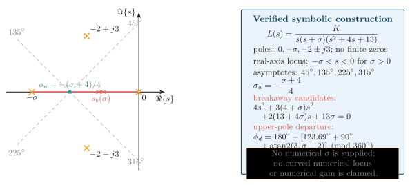
Source-faithful symbolic construction for the parameterized NTC 2081 root-locus problem. The real-axis segment and asymptotes are exact; horizontal marker positions are schematic because $\sigma$ is unspecified.

Note

Law — Source-paper limitation

The source paper prints the parameter $\sigma$, not a numeral, and provides no later numerical value. Consequently the exact breakaway coordinate, departure angle, gain labels, and curved branches must remain functions of $\sigma$. the figure is a verified symbolic construction and deliberately does not claim a numerical locus.

[!NOTE]

Example — Basic root-locus data

For

$$L(s)=\frac{K}{s(s+2)(s+4)},$$

the open-loop poles are $0,-2,-4$, there are no finite zeros, and the number of branches is $n=3$.

Apply the odd-count rule on each real-axis interval:

Interval	Singularities to the right	On locus?
$(-\infty,-4)$	3	Yes
$(-4,-2)$	2	No
$(-2,0)$	1	Yes
$(0,\infty)$	0	No

There are three asymptotes, with

$$\theta_q=\frac{(2q+1)180^\circ}{3} \quad\Longrightarrow\quad \boxed{\theta=60^\circ,180^\circ,300^\circ}.$$

The centroid is

$$\boxed{\sigma_a=\frac{0-2-4}{3}=-2.}$$

the figure also shows the valid breakaway and the $K=48$ imaginary-axis crossing.

[!NOTE]

Example — Breakaway point

For

$$L(s)=\frac{K}{s(s+4)},$$

the characteristic equation is

$$s(s+4)+K=0,$$

so

$$K(s)=-s(s+4)=-s^2-4s.$$

Therefore

$$\frac{dK}{ds}=-2s-4=0 \quad\Longrightarrow\quad \boxed{s=-2}.$$

The interval $(-4,0)$ has one pole to its right, and $K(-2)=4>0$, so this stationary point is a valid breakaway.

[!NOTE]

Example — Stability range using Routh

Find the stable range of $K$ for

$$s^3+6s^2+11s+6+K=0.$$

The Routh array is

$$\begin{array}{c|cc} s^3 & 1 & 11 \\ s^2 & 6 & 6+K \\ s^1 & \dfrac{6(11)-(6+K)}{6}=\dfrac{60-K}{6} & 0 \\ s^0 & 6+K & 0 \end{array}$$

All first-column elements are positive when

$$\frac{60-K}{6}>0 \Rightarrow K<60, \qquad 6+K>0 \Rightarrow K>-6.$$

Thus the full real-gain stability interval is

$$\boxed{-6<K<60}.$$

For the conventional positive-gain root locus,

$$\boxed{0<K<60},$$

while $K=0$ is also stable if zero gain is admitted. At $K=60$, the $s^1$ row becomes zero and the auxiliary equation from the $s^2$ row is

$$6s^2+66=0,$$

giving the crossing pair $s=\pm j\sqrt{11}$; the third pole is $-6$.

[!NOTE]

Example — Gain at a desired pole

For

$$L(s)=\frac{K}{s(s+2)},$$

find $K$ when a closed-loop pole is at $s=-1+j2$. The two denominator vectors have angles $116.565^\circ$ and $63.435^\circ$; hence the loop angle is $-180^\circ$, so the point passes the angle condition. The magnitude condition gives

$$K=\lvert s(s+2)\rvert.$$

At $s=-1+j2$,

$$\lvert s\rvert=\sqrt{(-1)^2+2^2}=\sqrt5, \qquad \lvert s+2\rvert=\lvert1+j2\rvert=\sqrt5.$$

Therefore

$$\boxed{K=\sqrt5\,\sqrt5=5}.$$

Indeed, $s^2+2s+5=0$ has roots $-1\pm j2$.

Quick Revision Table

Topic	Key result
Characteristic equation	$1+K G(s)H(s)=0$
Angle condition	$\angle G(s)H(s)=(2q+1)180^\circ$ when $G(s)H(s)$ excludes the adjustable $K$
Magnitude condition	$\lvert K G(s)H(s)\rvert=1$
Number of branches	Number $n$ of open-loop poles
Branch start	Open-loop poles at $K=0$
Branch end	Open-loop zeros or infinity as $K\to\infty$
Real-axis rule	Odd number of real poles and zeros to the right
Number of asymptotes	$n-m$
Asymptote angles	$\theta_q=(2q+1)180^\circ/(n-m)$
Centroid	$\sigma_a=(\sum p_i-\sum z_i)/(n-m)$
Break-point candidates	$dK/ds=0$, followed by segment and $K\ge0$ checks
Stability crossing	Routh–Hurwitz array and its auxiliary equation
Constant damping-ratio line	$\zeta=\cos\theta$
Constant natural-frequency line	$\lvert s\rvert=\omega_n$
Constant settling-time line	Vertical line $\Re\{s\}=-4/t_s$ under the $2\%$ approximation
Gain at a locus point	$K=\prod\lvert s-p_i\rvert/\prod\lvert s-z_i\rvert$

Root-locus results for rapid revision

Note

Key Point — Quick review

• Root locus shows closed-loop pole motion as $K$ varies from $0$ to $\infty$.

• Branches start at open-loop poles and end at open-loop zeros or infinity.

• A real-axis interval belongs to the $K\ge0$ locus when an odd number of real open-loop poles and zeros lie to its right.

• The angle condition decides membership; the magnitude condition then supplies gain.

• Routh–Hurwitz gives exact imaginary-axis crossings and stable gain inequalities.

• Design grids map pole location to $\zeta$, $\omega_n$, and settling time, but a target must still lie on the root locus.

• Adding a zero often improves relative stability, while adding a pole often reduces it; the full compensated angle condition is decisive.