FIR and IIR Filters

A digital filter processes a discrete-time signal to alter its frequency content. It passes desired components, attenuates unwanted components, or changes their relative phase. Every practical LTI digital filter is characterized equivalently by its difference equation, impulse response $h[n]$, system function $H(z)$, or frequency response $H(\mathrm{e}^{\mathrm{j}\Omega})$.

Digital angular frequency is normalized to the sampling frequency:

$$\Omega=2\pi\frac{f}{f_s} \quad\text{rad/sample}, \qquad f=\frac{\Omega}{2\pi}f_s.$$

The DT frequency response is $2\pi$-periodic, so a principal interval such as $-\pi\leq\Omega\leq\pi$ is sufficient. The point $\Omega=\pi$ corresponds to the Nyquist frequency $f_s/2$.

Ideal Frequency-Selective Filters

For a real zero-phase ideal response, the four basic magnitude specifications over $|\Omega|\leq\pi$ are

Caution

Key Formula — Ideal digital-filter definitions

$$\begin{aligned} \left\lvert H_{\mathrm{LP}}(\mathrm{e}^{\mathrm{j}\Omega})\right\rvert &=\begin{cases} 1,&0\leq\left\lvert \Omega\right\rvert\leq\Omega_c,\\ 0,&\Omega_c<\left\lvert \Omega\right\rvert\leq\pi, \end{cases}\\[1mm] \left\lvert H_{\mathrm{HP}}(\mathrm{e}^{\mathrm{j}\Omega})\right\rvert &=\begin{cases} 0,&0\leq\left\lvert \Omega\right\rvert<\Omega_c,\\ 1,&\Omega_c\leq\left\lvert \Omega\right\rvert\leq\pi, \end{cases}\\[1mm] \left\lvert H_{\mathrm{BP}}(\mathrm{e}^{\mathrm{j}\Omega})\right\rvert &=\begin{cases} 1,&\Omega_1\leq\left\lvert \Omega\right\rvert\leq\Omega_2,\\ 0,&\text{otherwise}, \end{cases}\\[1mm] \left\lvert H_{\mathrm{BS}}(\mathrm{e}^{\mathrm{j}\Omega})\right\rvert &=\begin{cases} 0,&\Omega_1<\left\lvert \Omega\right\rvert<\Omega_2,\\ 1,&\text{otherwise}. \end{cases} \end{aligned}$$

Thus a low-pass filter (LPF) passes low frequencies, a high-pass filter (HPF) passes high frequencies, a band-pass filter (BPF) passes only a selected band, and a band-stop or notch filter (BSF) rejects a selected band. The value assigned at a single cutoff point does not affect the inverse transform.

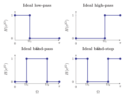
Ideal one-sided digital-filter magnitude responses over $0\leq\Omega\leq\pi$. The negative-frequency halves are obtained by even symmetry for real zero-phase responses.

Why a brick-wall ideal filter is noncausal

For the zero-phase ideal LPF,

$$H_{\mathrm{LP}}(\mathrm{e}^{\mathrm{j}\Omega})= \begin{cases} 1,&\left\lvert \Omega\right\rvert\leq\Omega_c,\\ 0,&\Omega_c<\left\lvert \Omega\right\rvert\leq\pi. \end{cases}$$

Applying the inverse DTFT gives

$$\begin{aligned} h_{\mathrm{LP}}[n] &=\frac{1}{2\pi}\int_{-\Omega_c}^{\Omega_c} \mathrm{e}^{\mathrm{j}\Omega n}\mathrm{d}\Omega\\ &=\begin{cases} \dfrac{\Omega_c}{\pi},&n=0,\\[2mm] \dfrac{\sin(\Omega_cn)}{\pi n},&n\neq0. \end{cases} \end{aligned}$$

This sinc-shaped sequence extends to both $n=+\infty$ and $n=-\infty$. Therefore it depends on future input samples and is noncausal. No finite delay can move an infinitely long negative-time tail entirely to $n\geq0$. The other ideal responses are combinations of ideal low-pass responses:

$$\begin{aligned} h_{\mathrm{HP}}[n] &=\delta[n]-h_{\mathrm{LP},\Omega_c}[n],\\ h_{\mathrm{BP}}[n] &=h_{\mathrm{LP},\Omega_2}[n]-h_{\mathrm{LP},\Omega_1}[n],\\ h_{\mathrm{BS}}[n] &=\delta[n]-h_{\mathrm{BP}}[n]. \end{aligned}$$

They inherit the same infinite two-sided support. Moreover, the $1/n$ tail of an exact brick-wall response is not absolutely summable in general, so the ideal zero-phase filter is not a causal BIBO-stable realization.

Practical filters replace the abrupt discontinuity by a transition band. A specification normally states passband edge $\Omega_p$, stopband edge $\Omega_s$, maximum passband ripple $\delta_p$, and maximum stopband level $\delta_s$. A narrower transition band or smaller allowed ripple requires a higher order, more computation, or both.

Tip

Exam Focus — Ideal-filter trap

An ideal rectangular magnitude response is a useful specification, not a physically realizable real-time filter. “Infinite impulse response” alone does not imply IIR recursion: the ideal zero-phase sinc is infinite and two-sided, whereas a realizable IIR filter is causal and recursive.

Finite Impulse Response Filters

An FIR filter has an impulse response of finite duration. A causal FIR filter of order $M$ and length $L=M+1$ obeys

Caution

Key Formula — FIR convolution and system function

$$\begin{aligned} y[n]&=\sum_{k=0}^{M}b_kx[n-k], \\ h[n]&=\begin{cases} b_n,&0\leq n\leq M,\\ 0,&\text{otherwise}, \end{cases} \\ H(z)&=\sum_{k=0}^{M}b_kz^{-k}. \end{aligned}$$

The output is the finite convolution of the input with the coefficient sequence. It depends only on present and past inputs, never on a past output, so the structure is non-recursive.

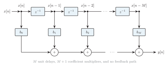
Generic FIR direct-form or transversal realization. The tapped delay line stores the present and past input samples and weights them by $b_0,\ldots,b_M$ before summation.

The direct or transversal realization is a tapped delay line. It uses $M$ unit delays, $M+1$ coefficient multipliers, and $M$ additions when all taps are nonzero. Each delay exposes another input sample, each multiplier forms $b_kx[n-k]$, and the adder chain forms the convolution sum.

For finite coefficients,

$$\sum_{n=-\infty}^{\infty}\left\lvert h[n]\right\rvert =\sum_{n=0}^{M}\left\lvert b_n\right\rvert<\infty.$$

Hence every such FIR filter is BIBO stable. In the $z$-plane its nontrivial finite zeros shape the response; poles introduced by writing the delay polynomial as a ratio are only at the origin and do not threaten causal stability.

Exact linear phase

An FIR filter with real coefficients has exact generalized linear phase when its impulse response is symmetric or antisymmetric about its midpoint:

Caution

Key Formula — FIR linear-phase coefficient conditions

$$\begin{aligned} h[n]&=h[M-n] &&\text{(symmetric)}, \\ h[n]&=-h[M-n] &&\text{(antisymmetric)}. \end{aligned}$$

Pairing samples equidistant from $M/2$ factors the frequency response as

$$H(\mathrm{e}^{\mathrm{j}\Omega}) =\mathrm{e}^{-\mathrm{j}\Omega M/2}A(\Omega),$$

where $A(\Omega)$ is real for symmetric coefficients and is purely imaginary apart from a constant $\mathrm{j}$ factor for antisymmetric coefficients. Therefore the phase is linear, apart from $\pi$ jumps where $A(\Omega)$ changes sign, and the group delay is constant:

$$\tau_g=-\frac{\mathrm{d}\angle H(\mathrm{e}^{\mathrm{j}\Omega})}{\mathrm{d}\Omega}=\frac{M}{2} \quad\text{samples}.$$

Symmetry also reduces arithmetic: paired samples can be added or subtracted before one shared multiplication.

The four real linear-phase FIR types are classified by symmetry and length.

Type	Coefficient relation	Length and order	Forced frequency-response zeros
I	Symmetric	$L$ odd, $M$ even	None at $0$ or $\pi$
II	Symmetric	$L$ even, $M$ odd	$H(\mathrm{e}^{\mathrm{j}\pi})=0$
III	Antisymmetric	$L$ odd, $M$ even	$H(1)=0$ and $H(\mathrm{e}^{\mathrm{j}\pi})=0$
IV	Antisymmetric	$L$ even, $M$ odd	$H(1)=0$

Four types of real-coefficient linear-phase FIR filters.

Type III has a zero center coefficient because antisymmetry requires $h[M/2]=-h[M/2]$. The forced-zero restrictions matter in selecting a type: for example, Type II cannot realize a high-pass response with nonzero gain at $\Omega=\pi$, and antisymmetric Types III and IV are suited to differentiators and Hilbert transformers rather than ordinary low-pass filters.

Note

Example — Three-Point Moving-Average FIR Filter

For equal weights $b_0=b_1=b_2=1/3$,

$$\boxed{y[n]=\frac13\left(x[n]+x[n-1]+x[n-2]\right)}.$$

Thus

$$\begin{aligned} h[n]&=\frac13\bigl(\delta[n]+\delta[n-1]+\delta[n-2]\bigr),\\ H(z)&=\frac13\left(1+z^{-1}+z^{-2}\right),\\ H(\mathrm{e}^{\mathrm{j}\Omega}) &=\frac13\left(1+\mathrm{e}^{-\mathrm{j}\Omega}+\mathrm{e}^{-\mathrm{j}2\Omega}\right)\\ &=\frac13\mathrm{e}^{-\mathrm{j}\Omega}\left(1+2\cos\Omega\right)\\ &=\frac13\mathrm{e}^{-\mathrm{j}\Omega} \frac{\sin(3\Omega/2)}{\sin(\Omega/2)}. \end{aligned}$$

The limiting value at $\Omega=0$ is $H(1)=1$, so DC passes unchanged. The zeros are at $z=\mathrm{e}^{\pm\mathrm{j}2\pi/3}$, producing notches at $\Omega=\pm2\pi/3$. Since the coefficients are symmetric, the phase is linear and the group delay is one sample.

For a unit-step input with zero prehistory,

$$y[n]=\begin{cases} 0,&n<0,\\ 1/3,&n=0,\\ 2/3,&n=1,\\ 1,&n\geq2. \end{cases}$$

The averaging action suppresses rapid sample-to-sample changes, so this FIR acts as a low-pass smoothing filter.

FIR characteristics and applications

• No feedback: The realization is non-recursive and cannot sustain a zero-input limit cycle.

• Guaranteed stability: Finite coefficients give an absolutely summable finite impulse response.

• Phase control: Coefficient symmetry or antisymmetry gives exact linear phase and constant group delay.

• Main cost: A sharp transition generally requires a higher order, more delays, and more multiplications than an IIR design.

• Finite-word behavior: Coefficient quantization moves zeros and changes ripple, but there are no feedback poles to move outside the unit circle; round-off errors do not circulate indefinitely.

Typical FIR applications are linear-phase audio processing, communication pulse shaping and matched filtering, moving-average smoothing, multirate decimation/interpolation, and any design in which guaranteed stability or an undistorted waveform shape is more important than minimum order.

Infinite Impulse Response Filters

An IIR filter uses feedback. Its present output depends on present and past inputs and on past outputs:

Caution

Key Formula — General IIR difference equation and system function

$$\begin{aligned} y[n] &=\sum_{m=0}^{M}b_mx[n-m] -\sum_{k=1}^{N}a_ky[n-k], \\ H(z) &=\frac{\sum_{m=0}^{M}b_mz^{-m}} {1+\sum_{k=1}^{N}a_kz^{-k}}. \end{aligned}$$

The denominator creates recursive modes. After an impulse has entered, a nonzero pole generally causes the response to continue indefinitely, even when all subsequent input samples are zero. Degenerate exact cancellations can shorten the external impulse response, but they should not be relied upon to remove an internal unstable mode.

For a causal rational IIR filter, BIBO stability requires every pole of the reduced $H(z)$ to lie strictly inside the unit circle. A pole on the unit circle is not BIBO stable, and a pole outside it produces a growing causal natural response. As established in the section, that pole-only shorthand assumes the causal ROC outside the outermost pole.

IIR Direct-Form Realizations

Let

$$B(z)=\sum_{m=0}^{M}b_mz^{-m}, \qquad A(z)=1+\sum_{k=1}^{N}a_kz^{-k}, \qquad H(z)=\frac{B(z)}{A(z)}.$$

Delays, coefficient multipliers, and summers can realize this ratio in several mathematically equivalent ways. Internal signal ranges and finite-word sensitivity, however, need not be equivalent.

Direct Form I: separate delay lines

Direct Form I implements the original recursion directly. The feedforward part stores $x[n-m]$, while a separate feedback line stores $y[n-k]$. For a second-order example,

$$\begin{aligned} y[n]={}&b_0x[n]+b_1x[n-1]+b_2x[n-2]\\ &{}-a_1y[n-1]-a_2y[n-2]. \end{aligned}$$

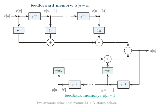
IIR Direct Form I realization. The numerator taps $b_0,\ldots,b_M$ use delayed input samples, while the signed denominator taps $-a_1,\ldots,-a_N$ use a separate delayed-output line.

The general DF-I realization uses $M+N$ delays, $M+1$ feedforward multipliers, and $N$ feedback multipliers. Its separate sections use more memory than the canonical form, but the separation can give more convenient internal scaling and can reduce overflow risk at a single shared state node.

Direct Form II: shared state delay line

Factor the system as an all-pole section followed by a feedforward section and define the intermediate state $w[n]$:

Caution

Key Formula — Direct Form II state equations

$$\begin{aligned} w[n]&=x[n]-\sum_{k=1}^{N}a_kw[n-k], \\ y[n]&=\sum_{m=0}^{M}b_mw[n-m]. \end{aligned}$$

Taking the $Z$-transform with zero initial state confirms

$$W(z)=\frac{X(z)}{A(z)}, \qquad Y(z)=B(z)W(z), \qquad \frac{Y(z)}{X(z)}=\frac{B(z)}{A(z)}.$$

The same delayed values $w[n-k]$ serve both sums, so the two lines merge. Coefficients missing when $M\neq N$ are treated as zero.

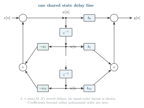
IIR Direct Form II, the canonical realization. Feedback taps $-a_1,\ldots,-a_N$ and feedforward taps $b_0,\ldots,b_M$ use the same stored states $w(n-k)$, reducing the memory to $\max(M,N)$ delays.

DF-II uses only $\max(M,N)$ delays and is therefore called the canonical direct form. For the usual case $M\leq N$, it uses $N$ state delays. Its economy comes with a numerical trade-off: the internal $w[n]$ can be much larger than the input or output because pole amplification occurs before numerator attenuation. Careful scaling is therefore more important than in DF-I.

Order, state, and delay count

For the coefficient form in the equation, the numerator order is $M$, the denominator order is $N$, and the direct realization order is normally $\max(M,N)$ after leading zero coefficients and common factors are removed. “FIR order $M$” means $M$ delays but $M+1$ taps; this common off-by-one distinction is exam-relevant.

Realization	Unit delays	Multipliers	Main structural fact
FIR direct form	$M$	$M+1$	One tapped input delay line; no feedback
IIR Direct Form I	$M+N$	$M+N+1$	Separate input and output delay lines
IIR Direct Form II	$\max(M,N)$	$M+N+1$	Shared state line; minimum delay memory

Delay and arithmetic counts for direct realizations with nonzero coefficients.

High-order IIR filters are rarely implemented as one large direct-form polynomial in finite precision. Factoring $H(z)$ into first- and second-order sections (SOS or biquads), ordering the sections, and scaling between them usually gives much better numerical robustness. Transposed direct forms realize the same transfer function with different internal round-off and overflow behavior.

Note

Example — First-Order IIR Smoothing Filter

Consider

$$y[n]=\frac12x[n]+\frac12y[n-1], \qquad y[-1]=0.$$

In the standard sign convention this is $y[n]-\tfrac12y[n-1]=\tfrac12x[n]$, so $a_1=-1/2$ and the actual feedback multiplier is $-a_1=+1/2$. With zero initial state,

$$\begin{aligned} Y(z)&=\frac12X(z)+\frac12z^{-1}Y(z),\\ \boxed{H(z)}&=\boxed{\frac{1/2}{1-(1/2)z^{-1}}},\\ h[n]&=\frac12\left(\frac12\right)^nu[n]. \end{aligned}$$

The only pole is $z=1/2$, so the causal filter is BIBO stable. Its frequency response magnitude is

$$\left\lvert H(\mathrm{e}^{\mathrm{j}\Omega})\right\rvert =\frac{1/2}{\sqrt{1+(1/2)^2-2(1/2)\cos\Omega}} =\frac{1/2}{\sqrt{1.25-\cos\Omega}}.$$

Therefore $|H(1)|=1$ at DC and $|H(\mathrm{e}^{\mathrm{j}\pi})|=1/3$ at the Nyquist frequency: it is a simple low-pass smoother, not an ideal brick-wall filter.

For $x[n]=u[n]$, either convolution or the first-order result from the previous section gives

$$\boxed{y[n]=1-\left(\frac12\right)^{n+1}},\qquad n\geq0.$$

The first samples are $1/2,3/4,7/8,15/16,\ldots$, approaching the final value $1$ while retaining an infinite decaying tail.

Finite-Word Effects in FIR and IIR Filters

Real implementations quantize coefficients, products, and stored states. Their consequences differ sharply because IIR errors circulate through feedback.

• Coefficient quantization: FIR zeros move and the magnitude ripple changes, but stability remains guaranteed. IIR poles also move; a pole close to $|z|=1$ can cross outside and make the quantized filter unstable.

• Round-off noise: An FIR arithmetic error passes through a finite path and dies out. In an IIR filter it is fed back and can be amplified or spectrally shaped by the poles.

• Limit cycles: Quantization makes an IIR recursion nonlinear. Even with $x[n]=0$, rounding or overflow can sustain a periodic zero-input oscillation. FIR filters without feedback do not have this autonomous limit-cycle mechanism.

• Overflow: Two’s-complement wraparound can create large errors or overflow limit cycles. Saturation arithmetic is usually less destructive but is still nonlinear.

Common IIR precautions are SOS implementation, section ordering, state scaling, guard bits, higher coefficient precision, saturation arithmetic, and rounding instead of truncation. Dither can suppress some small-amplitude deterministic cycles at the cost of added noise. Stability must be checked using the quantized coefficients, not only the ideal design values.

FIR and IIR Comparison

Feature	FIR filter	IIR filter
Impulse response	Finite duration	Theoretically infinite duration
Difference equation	Feedforward finite convolution	Feedforward plus recursive feedback
Structure	Non-recursive	Recursive
Feedback	None	Uses past outputs or internal states
Stability	Always BIBO stable for finite coefficients	Depends on pole locations; causal poles must satisfy $
Phase	Exact linear phase is possible by symmetry or antisymmetry	Generally nonlinear phase; exact causal linear phase is not normally possible for a nontrivial stable IIR
Order for a sharp cutoff	Usually higher	Usually lower
Computation	More multiplications for the same magnitude specification	Fewer multiplications and delays for a comparable sharp response
Quantization sensitivity	Lower; errors do not recur	Higher; pole movement and feedback amplify finite-word effects
Limit cycles	No feedback-induced zero-input limit cycles	Round-off or overflow limit cycles are possible
Typical design route	Windowing, frequency sampling, or optimal/equiripple design	Digital design or transformation of an analog prototype
Principal advantage	Guaranteed stability and controllable exact linear phase	Sharp transition with low order and low arithmetic cost
Principal limitation	Higher order, memory, computation, and delay	Possible instability, nonlinear phase, and finite-word sensitivity

Exam-oriented comparison of FIR and IIR digital filters.

Design and Application Notes

FIR design routes

An ideal impulse response can be truncated and multiplied by a window. The window length controls transition width; the window shape trades main-lobe width against stopband sidelobes. Frequency-sampling methods prescribe samples of the desired response, while equiripple methods distribute the worst-case weighted error optimally across bands. Increasing order generally narrows the transition, but also increases group delay $M/2$ for a linear-phase design.

Choose an FIR filter when waveform shape and phase linearity matter, when stability must be unconditional, or when multirate/polyphase implementation can exploit many zero coefficients. Representative uses include audio and image processing, data-communication pulse shaping, channel equalization, matched filtering, and moving-average sensor smoothing.

IIR design routes

IIR filters are often obtained from stable analog prototypes. A Butterworth prototype is maximally flat in the passband; a Chebyshev prototype accepts ripple for a sharper transition; an elliptic prototype allows ripple in both passband and stopband for a still lower order. The bilinear transform avoids aliasing but warps frequency and may require prewarping. Impulse invariance maps sampled analog impulse responses but can alias analog spectral copies.

Choose an IIR filter when arithmetic, memory, latency, or processor power is limited and exact linear phase is unnecessary. Applications include low-order real-time audio equalizers and tone controls, speech and communication-channel filtering, biomedical low-pass/high-pass/notch filtering, recursive sensor smoothing, and digital Butterworth, Chebyshev, or elliptic filters.

Tip

Exam Focus — Digital-filter exam traps

1. Do not confuse FIR order $M$ with length $M+1$.

2. FIR stability follows from finite $h[n]$ and finite coefficients; exact linear phase additionally requires coefficient symmetry or antisymmetry.

3. In $y[n]+\sum a_ky[n-k]=\sum b_mx[n-m]$, the feedback multiplier is $-a_k$. Read the sign before drawing a realization.

4. For a causal IIR filter, poles must lie strictly inside the unit circle; zeros do not determine BIBO stability.

5. DF-I and DF-II realize the same $H(z)$ but not the same internal numerical ranges. DF-II is canonical because it shares the state line.

6. A pole–zero cancellation can hide an unstable internal mode and is unreliable after coefficient quantization.

7. Convert hertz to normalized frequency before evaluating $H(\mathrm{e}^{\mathrm{j}\Omega})$, and remember that $\Omega=\pi$ means $f_s/2$.

8. Ideal brick-wall LP/HP/BP/BS responses are noncausal specifications; every realizable design has a transition band.

[!NOTE]

Key Point — Quick Review

Differential equations map to $H(s)$ and difference equations map to $H(z)$, both under zero initial conditions. FIR filters have finite $h[n]$, no feedback, guaranteed stability, and possible exact linear phase, but normally need higher order. IIR filters use feedback and give sharp responses with fewer coefficients, delays, and multiplications, but causal stability depends on all poles being strictly inside the unit circle. Direct Form II shares one state delay line and therefore uses the minimum number of delays.