Antennas and Polarization

Chapter Overview

ANTENNAS
|
|-- Antenna fundamentals
|   |-- Radiation and field regions
|   |-- Radiation pattern and beamwidth
|   |-- Directivity and gain
|   |-- Efficiency and radiation resistance
|   `-- Effective aperture and Friis equation
|
|-- Polarization
|   |-- Linear polarization
|   |-- Circular polarization
|   |-- Elliptical polarization
|   `-- Polarization mismatch
|
`-- Dipole antenna
  |-- Hertzian current element
  |-- Practical short dipole
  |-- Half-wave dipole
  |-- Radiation patterns
  `-- Radiation resistance

Antenna Radiation

Note

Antenna.

An antenna is a transducer that converts guided electromagnetic energy into free-space electromagnetic waves during transmission, and converts received free-space electromagnetic waves into guided electrical energy during reception.

• In transmission, it converts terminal voltage and current into radiated fields.

• In reception, it intercepts an incident field and produces terminal voltage and current.

• For a linear, passive antenna, the transmitting and receiving properties are reciprocal: the same pattern, directivity and polarization apply in both modes.

Why an antenna radiates

Note

Antenna radiation.

Antenna radiation is the outward transport of electromagnetic energy by the non-cancelling $1/r$ fields produced by accelerating charge, equivalently by a time-varying current distribution having a non-zero radiation moment.

• A static charge produces an electrostatic field and a steady current produces a magnetostatic field, but neither produces a time-varying $1/r$ field that continuously transports energy to infinity.

Note

Radiation-mechanism vocabulary.

• Geometrical deformation: bending or flaring conductors so opposite current elements are no longer closely superposed and their far fields no longer cancel completely.

• Electrical discontinuity: an open end, bend, junction or abrupt structural change at which the guided current distribution must change.

• Local unbalanced charge: alternating charge separation caused by a non-zero current gradient; total charge of the complete antenna-source system remains conserved.

Balanced line and field cancellation

• On a closely spaced uniform two-wire line, the conductors carry approximately equal and opposite currents: $I_1(z,t)=-I_2(z,t)$.

• When conductor spacing $s\ll\lambda$, corresponding current elements are close together and oppositely directed. Their distant fields therefore nearly cancel: $\mathbf E_{\mathrm{far,total}}\approx\mathbf E_1+\mathbf E_2\approx0$.

• Most electromagnetic energy remains confined around and between the conductors as a guided wave. A practical line still radiates slightly at bends, junctions and imperfectly balanced sections, but an ideal uniform balanced line is a poor radiator.

Geometrical deformation: bending or flaring the wires

• When the two conductors are bent or flared outward to form a dipole, this geometrical deformation changes the positions and directions of the current elements. The opposite-current elements are no longer so closely superposed, so their fields do not cancel in every far-zone direction:

$$\mathbf E_{\mathrm{far,total}} =\mathbf E_1+\mathbf E_2\ne0.$$

• The separated current distribution consequently has a non-zero electric-dipole moment and can radiate. Bending is a useful transmission-line-to-dipole picture, but it is not itself the fundamental cause: any suitable time-varying current distribution, including that on a straight dipole, radiates when its far fields do not cancel.

Electrical discontinuity and local unbalanced charge

• Each open wire end is an electrical discontinuity. Conduction current cannot continue into free space, so the thin-wire current satisfies the boundary condition $I\!\left(\pm\frac{\ell}{2},t\right)=0$.

• Current and charge cannot vary independently. Conservation of charge requires $\nabla\cdot\mathbf J =-\frac{\partial\rho_v}{\partial t}$

• or, for a thin wire with line-charge density $\lambda_q(z,t)$,

$$\boxed{ \frac{\partial I(z,t)}{\partial z} =-\frac{\partial\lambda_q(z,t)}{\partial t} }.$$

• Because $I$ varies along the wire and falls to zero at an open end, $\partial I/\partial z\ne0$ and alternating surface charge accumulates. During one half-cycle one arm has excess positive charge while the other has excess negative charge; the polarities reverse during the next half-cycle. These are locally unbalanced charges, or charge separation. The total charge of the complete isolated antenna-plus-source system remains conserved.

• For sinusoidal steady state, $dI/dz=-j\omega\lambda_q$, so a large current gradient corresponds directly to a large alternating charge density. Current is generally largest near a centre feed and zero at the tips, whereas charge is strongest near the open ends.

Time-varying fields become a radiation field

• The alternating charge produces a time-varying electric field, and the alternating current produces a time-varying magnetic field. Maxwell’s curl equations couple them:

$$\nabla\times\mathbf E=-\frac{\partial\mathbf B}{\partial t}, \qquad \nabla\times\mathbf H =\mathbf J+\frac{\partial\mathbf D}{\partial t}.$$

• Changes in the source are not communicated instantaneously. The fields at observation point $\mathbf r$ depend on charge and current at the retarded time

$$t_r=t-\frac{R}{v}, \qquad R=|\mathbf r-\mathbf r'|.$$

• For example, the magnetic vector potential is

$$\mathbf A(\mathbf r,t) =\frac{\mu}{4\pi} \iiint_V \frac{\mathbf J(\mathbf r',t-R/v)}{R}\,dV'.$$

• Because different parts of a finite antenna are at different positions and have different current directions and retarded phases, their radiation contributions do not cancel everywhere. For an electrically short $z$-directed source, the surviving far fields have the form. where,

$$\boxed{ E_\theta =j\eta\frac{kI_0\ell_{\mathrm{eff}}}{4\pi r} e^{-jkr}\sin\theta, \qquad H_\phi=\frac{E_\theta}{\eta} },$$ $$\ell_{\mathrm{eff}} =\frac{1}{I_0}\int I(z)\,dz$$

• is the effective current length. The non-zero $1/r$ term is the radiation field: it is maximum broadside to the current and zero along the wire axis.

• The common phrase that field lines detach or pinch off is a useful visualization, not a separate event in Maxwell’s equations. The fields evolve continuously from source-bound near fields into a propagating $1/r$ component; no physical field line breaks at a sharply defined boundary.

• The field of a finite source contains terms proportional to $\frac{1}{r^3},\frac{1}{r^2}, \frac{1}{r}.$

Distance dependence	Main interpretation
$1/r^3$	reactive electric-field storage near the antenna
$1/r^2$	induction and transition field
$1/r$	radiation field; this term dominates far from the antenna

• Although the far electric and magnetic fields each fall as $1/r$, their power density falls as $1/r^2$. The area of a sphere grows as $4\pi r^2$, so the total power crossing the sphere remains constant.

• For an outward travelling wave in a lossless medium,

$$\mathbf H=\frac{1}{\eta}\hat{\mathbf r}\times\mathbf E, \qquad \mathbf E\perp\mathbf H\perp\hat{\mathbf r},$$

• where $\eta=\sqrt{\mu/\varepsilon}$ is the intrinsic impedance. The time-average Poynting vector is

$$\mathbf S_{\mathrm{av}} =\frac{1}{2}\operatorname{Re}\!\left(\mathbf E\times\mathbf H^*\right) =\hat{\mathbf r}\frac{|\mathbf E|^2}{2\eta} \quad\text{W/m}^2,$$

• when peak-value phasors are used.

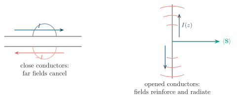
Transition from a guided two-wire wave to dipole radiation.

• On the uniform two-wire line, equal and opposite currents produce distant fields that nearly cancel. Flaring the wires introduces geometrical deformation, separates the opposite currents and reduces cancellation. The open ends introduce discontinuities where current becomes zero and alternating charge is greatest. The resulting distributed current and charge produce the non-cancelled $1/r$ field of a centre-fed dipole.

Antenna field regions

Note

Antenna field regions.

The reactive near field is dominated by stored energy, the radiating near field or Fresnel region contains outward radiation whose angular distribution still depends on distance, and the far field or Fraunhofer region has locally transverse fields and a distance-independent angular pattern.

Let $D_a$ be the largest physical dimension of the antenna and let $\lambda$ be the wavelength. Common engineering boundaries are

$$\begin{aligned} \text{Reactive near field:}\quad & r < 0.62\sqrt{\frac{D_a^3}{\lambda}}, \\[2mm] \text{Radiating near field (Fresnel):}\quad & 0.62\sqrt{\frac{D_a^3}{\lambda}} \le r < \frac{2D_a^2}{\lambda}, \\[2mm] \text{Far field (Fraunhofer):}\quad & r \ge \frac{2D_a^2}{\lambda}. \end{aligned}$$

These are practical estimates, especially for antennas large compared with a wavelength.

Note

Far-field boundary

An antenna with maximum dimension $D_a=2\ \mathrm m$ operates at $300\ \mathrm{MHz}$, for which $\lambda=1\ \mathrm m$. Its usual Fraunhofer-distance estimate is

$$R_{\text{FF}}=\frac{2D_a^2}{\lambda} =\frac{2(2)^2}{1}=8\ \mathrm m.$$

Far-field pattern or gain measurements should therefore be made at $R\ge8\ \mathrm m$, with additional separation when the measurement geometry requires it.

Feature	Reactive near field	Radiating near field (Fresnel)	Far field (Fraunhofer)
Dominant energy behavior	Stored electric or magnetic energy dominates and is exchanged with the antenna each cycle; little net outward power may cross a nearby closed surface.	Outward radiated power is significant, but field amplitude and phase still depend on both angle and distance.	The outward radiation term dominates; reactive stored-field terms are negligible compared with radiated power.
Important distance terms	$1/r^3$ reactive and $1/r^2$ induction terms are important.	The $1/r$ radiation term is important, but residual near-field terms and aperture phase differences still affect the field.	Fields vary approximately as $1/r$, and average power density varies as $1/r^2$.
Electric and magnetic fields	$\mathbf E$ and $\mathbf H$ need not be in phase, transverse or related by $E/H=\eta$; either electric or magnetic energy may dominate.	$\mathbf E$ and $\mathbf H$ approach radiation-field behavior but can retain longitudinal components and a position-dependent ratio.	In a lossless medium, $\mathbf E$ and $\mathbf H$ are approximately in phase, mutually perpendicular and transverse to $\hat{\mathbf r}$, with $E/H=\eta$.
Wavefront	Strongly curved and coupled to source geometry.	Curved; different parts of a large aperture can have appreciably different path lengths to the observation point.	Locally plane over a receiving aperture; rays are approximately parallel.
Radiation pattern	No unique distance-independent radiation pattern; small probe movements can strongly change measured amplitude and phase.	Pattern shape changes with $r$, and lobes and nulls continue to develop with distance.	Normalized angular pattern is stable and independent of $r$; only its common $1/r$ field scale changes.
Practical significance	Nearby objects can store energy with the antenna, alter input impedance and detune it.	Fresnel diffraction and aperture geometry must be included in measurements or links.	Standard gain, directivity, polarization and radiation-pattern measurements are valid.
Approximate radial range	$r<0.62\sqrt{D_a^3/\lambda}$	$0.62\sqrt{D_a^3/\lambda}\le r<2D_a^2/\lambda$	$r\ge2D_a^2/\lambda$

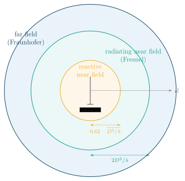
Antenna field regions.

How to read the figure. The concentric boundaries represent changes in field behavior, not physical shells. Near the antenna, energy is repeatedly stored and returned to the source. In the Fresnel region, energy travels outward but the pattern depends on distance. Beyond the far-field boundary, rays are approximately parallel over the receiving aperture and only the common $1/r$ scale factor changes with distance.

Radiation Pattern

Note

Radiation pattern.

A radiation pattern is the angular variation of radiated field or power at a fixed, sufficiently large radius. A complete pattern is three-dimensional, but it is usually shown using two principal-plane cuts.

Principal pattern planes.

• The E-plane contains the electric-field vector and the direction of maximum radiation.

• The H-plane contains the magnetic-field vector and the direction of maximum radiation.

Normalized patterns. A normalized field pattern is field magnitude divided by its maximum value; a normalized power pattern is the corresponding power divided by its maximum value.

If $F(\theta,\phi)$ is a field-pattern function, its normalized magnitude is

$$F_n(\theta,\phi) =\frac{|F(\theta,\phi)|}{|F|_{\max}}.$$

Because power is proportional to the square of field magnitude, the normalized power pattern is

$$P_n(\theta,\phi)=|F_n(\theta,\phi)|^2.$$

The same pattern expressed in decibels is

$$P_n\big|_{\mathrm{dB}} =10\log_{10}P_n =20\log_{10}F_n.$$

Pattern terminology

Note

Pattern terminology.

The table defines the lobes, nulls, beamwidths and side-lobe level used to describe a radiation pattern.

Term	Meaning
Main lobe	lobe containing the direction of maximum radiation
Side lobe	unwanted lobe adjacent to the main lobe
Back lobe	lobe approximately opposite the main beam
Null	direction in which ideal radiation is zero
HPBW	angle between the two half-power points of the main lobe
FNBW	angle between the first nulls surrounding the main lobe
Side-lobe level	peak side-lobe power relative to the main-lobe peak, in dB

At a half-power point,

$$P_n=\frac{1}{2}, \qquad F_n=\frac{1}{\sqrt2}=0.707, \qquad P_n\big|_{\mathrm{dB}}=-3.01\ \mathrm{dB}.$$

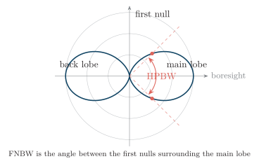
Radiation-pattern terminology and half-power beamwidth.

How to read the figure. Radius represents normalized radiated power, while angle represents direction. The boresight axis passes through the main-lobe maximum. The two marked $-3$ dB directions enclose the HPBW; the null directions enclose the wider FNBW. A narrower main beam usually indicates greater directivity, but side- and back-lobe power must also be included when total radiated power is calculated.

Radiation Intensity and Total Radiated Power

Note

Radiation intensity.

Radiation intensity $U$ is power radiated per unit solid angle. In the far field it removes the $1/r^2$ distance dependence from radial power density: $U=r^2S_r$.

In the far field, radial power density has the form $S_r\propto1/r^2$:

$$U(\theta,\phi)=r^2S_r(\theta,\phi) \quad\text{W/sr}.$$

The power radiated into a solid-angle element is

$$dP_{\mathrm{rad}}=U(\theta,\phi)d\Omega, \qquad d\Omega=\sin\theta\,d\theta\,d\phi.$$

Therefore,

$$P_{\mathrm{rad}} =\int_{0}^{2\pi}\int_{0}^{\pi} U(\theta,\phi)\sin\theta\,d\theta\,d\phi.$$

Note

Isotropic radiator.

An isotropic radiator is an ideal point reference that radiates equally in every direction. It is not physically realizable.

For an isotropic radiator,

$$U_0=\frac{P_{\mathrm{rad}}}{4\pi}.$$

Directivity

Note

Directivity.

Directivity compares radiation intensity in a specified direction with the average intensity of an isotropic radiator radiating the same total power.

$$D(\theta,\phi) =\frac{U(\theta,\phi)}{U_0} =\frac{4\pi U(\theta,\phi)}{P_{\mathrm{rad}}}.$$

The maximum directivity is

$$D_0=\frac{4\pi U_{\max}}{P_{\mathrm{rad}}}.$$

Note

Beam solid angle.

The beam solid angle $\Omega_A$ is the solid angle through which all radiation would flow if radiation intensity were constant at its maximum value; equivalently, it is the integral of the normalized power pattern over $4\pi$ steradians.

If $P_n$ is the normalized power pattern,

$$\Omega_A=\int_{4\pi}P_n(\theta,\phi)d\Omega,$$

and hence

$$D_0=\frac{4\pi}{\Omega_A}.$$

Directivity is dimensionless. Relative to an isotropic radiator,

$$D_{\mathrm{dBi}}=10\log_{10}D.$$

Antenna directivity redistributes power; it does not create power.

Gain and Efficiency

Note

Gain.

Antenna gain is directivity reduced by radiation loss: $G=\eta_rD$. Directivity depends only on pattern shape, whereas gain also accounts for power dissipated inside the antenna.

$$G(\theta,\phi)=\eta_rD(\theta,\phi), \qquad G_0=\eta_rD_0,$$

Note

Radiation efficiency.

Radiation efficiency $\eta_r$ is the fraction of accepted terminal power that is radiated rather than dissipated as conductor or dielectric loss.

$$\eta_r=\frac{P_{\mathrm{rad}}}{P_{\mathrm{acc}}} =\frac{P_{\mathrm{rad}}} {P_{\mathrm{rad}}+P_{\mathrm{loss}}}.$$

Here $P_{\mathrm{acc}}$ is power accepted at the antenna terminals. If conductor and dielectric loss are represented by $R_{\mathrm{loss}}$,

$$\eta_r=\frac{R_r}{R_r+R_{\mathrm{loss}}}.$$

Note

Total efficiency and realized gain.

Total efficiency $\eta_0$ includes both radiation loss and terminal mismatch. Realized gain is directivity multiplied by total efficiency.

If terminal mismatch is also included,

$$\eta_0=(1-|\Gamma_A|^2)\eta_r, \qquad G_{\mathrm{realized}}=\eta_0D,$$

where

$$\Gamma_A=\frac{Z_A-Z_0}{Z_A+Z_0}$$

for a real feed-line impedance $Z_0$.

The decibel forms are

$$G_{\mathrm{dBi}}=10\log_{10}G, \qquad G_{\mathrm{dBd}}=G_{\mathrm{dBi}}-2.15\ \mathrm{dB},$$

because a lossless half-wave dipole has approximately $2.15$ dBi directivity.

Radiation Resistance and Input Impedance

Note

Radiation resistance.

Radiation resistance $R_r$ is the equivalent resistance that would dissipate the same power as the antenna radiates. It is not a physical resistor and does not represent heat loss.

For RMS terminal current,

$$P_{\mathrm{rad}}=I_{\mathrm{rms}}^2R_r.$$

For a peak-current phasor $I_0$,

$$P_{\mathrm{rad}}=\frac{1}{2}|I_0|^2R_r.$$

Note

Antenna input impedance.

Antenna input impedance $Z_A$ is the ratio of terminal voltage to terminal current. Its real part contains radiation and loss resistance, while its imaginary part represents net stored electric or magnetic energy.

The input impedance is

$$Z_A=R_A+jX_A =(R_r+R_{\mathrm{loss}})+jX_A.$$

Part	Physical meaning
$R_r$	useful power carried away as radiation
$R_{\mathrm{loss}}$	conductor and dielectric heating
$X_A$	net stored electric or magnetic energy near the antenna

At resonance, $X_A=0$. Matching the resonant resistance to the feed line minimizes reflected power; it does not by itself remove conductor or dielectric loss.

Effective Aperture

Note

Effective aperture.

Effective aperture, or effective area, is the equivalent receiving area that relates incident power density to the maximum available received power under conjugate impedance and polarization matching.

If the incident time-average power density is $S_{\mathrm{inc}}$, then

$$P_{r,\max}=S_{\mathrm{inc}}A_e.$$

The maximum effective aperture and gain are related by

$$A_{e,\max}=\frac{\lambda^2G_0}{4\pi}.$$

Thus effective aperture is not necessarily the antenna’s physical area. A thin dipole has almost no geometric capture area but has a finite effective aperture.

For an isotropic receiving antenna,

$$A_{e,\mathrm{iso}}=\frac{\lambda^2}{4\pi}.$$

Friis Free-Space Transmission Equation

Note

Friis free-space transmission equation.

The Friis equation relates received power to transmitted power, antenna gains, wavelength and separation for matched, polarization-aligned antennas in each other’s far field under unobstructed free-space conditions.

At distance $R$ in the transmitting antenna’s far field, the power density on boresight is

$$S_t=\frac{P_tG_t}{4\pi R^2}.$$

Using $P_r=S_tA_{e,r}$ and $A_{e,r}=\lambda^2G_r/(4\pi)$ gives the Friis equation:

$$\boxed{ P_r=P_tG_tG_r \left(\frac{\lambda}{4\pi R}\right)^2 }$$

for matched, polarization-aligned antennas in unobstructed free space. Including polarization mismatch,

$$P_r=P_tG_tG_r \left(\frac{\lambda}{4\pi R}\right)^2 \mathrm{PLF}.$$

Note

Free-space path loss.

Free-space path loss $L_{\mathrm{fs}}$ is the ideal spreading loss between isotropic antennas in unobstructed free space, excluding antenna, feeder, polarization and atmospheric losses.

Its linear ratio is

$$L_{\mathrm{fs}}= \left(\frac{4\pi R}{\lambda}\right)^2,$$

or

$$L_{\mathrm{fs,dB}} =20\log_{10}\!\left(\frac{4\pi R}{\lambda}\right).$$

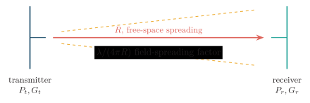
Quantities in the Friis free-space link.

How to read the figure. The transmitting gain $G_t$ concentrates $P_t$ into the receiving direction. Spherical spreading reduces power density by $1/(4\pi R^2)$. The receiving antenna then captures the fraction represented by its effective aperture $A_{e,r}$. Friis combines these three steps; it applies to far-field, line-of-sight propagation and does not include ground reflection, obstruction, atmospheric loss or feeder loss unless separate factors are added.

Summary

Quantity	Meaning
Radiation pattern	angular distribution of field or power
Radiation intensity $U$	power per unit solid angle, $U=r^2S_r$
Directivity $D$	pattern concentration relative to an isotropic radiator
Gain $G$	directivity including radiation efficiency, $G=\eta_rD$
Radiation efficiency $\eta_r$	$P_{\mathrm{rad}}/P_{\mathrm{acc}}$
Radiation resistance $R_r$	equivalent resistance representing radiated power
Effective aperture $A_e$	equivalent receiving area, $A_e=\lambda^2G/(4\pi)$

Worked example: directivity, gain and aperture

An antenna has maximum directivity $D_0=6$, radiation efficiency $\eta_r=80\%$, and operates at $300$ MHz. Find its gain and maximum effective aperture.

First,

$$\lambda=\frac{c}{f} =\frac{3\times10^8}{300\times10^6} =1\ \mathrm m.$$

Then,

$$G_0=\eta_rD_0=0.8(6)=4.8,$$ $$G_{0,\mathrm{dBi}}=10\log_{10}(4.8)=6.81\ \mathrm{dBi},$$

and

$$A_{e,\max}=\frac{\lambda^2G_0}{4\pi} =\frac{1^2(4.8)}{4\pi} =0.382\ \mathrm{m}^2.$$

Polarization

Note

Polarization.

Polarization describes the orientation and time variation of the electric-field vector of a wave at a fixed point in space. The magnetic field is perpendicular to the electric field, but antenna polarization is defined using $\mathbf E$.

For a uniform plane wave travelling in the $+z$ direction, write the two transverse components as

$$\mathbf E(z,t) =\hat{\mathbf x}E_{x0}\cos(\omega t-\beta z) +\hat{\mathbf y}E_{y0}\cos(\omega t-\beta z+\delta),$$

where

• $E_{x0}$ and $E_{y0}$ are non-negative component amplitudes;

• $\delta$ is the phase of the $y$ component relative to the $x$ component;

• polarization is found by holding $z$ fixed and observing the tip of $\mathbf E$ as $t$ changes.

The corresponding electric-field phasor is

$$\widetilde{\mathbf E}(z) =\left(\hat{\mathbf x}E_{x0} +\hat{\mathbf y}E_{y0}e^{j\delta}\right)e^{-j\beta z}.$$

Eliminating time from the two instantaneous components gives

$$\left(\frac{E_x}{E_{x0}}\right)^2 +\left(\frac{E_y}{E_{y0}}\right)^2 -2\left(\frac{E_x}{E_{x0}}\right) \left(\frac{E_y}{E_{y0}}\right)\cos\delta =\sin^2\delta.$$

This is generally an ellipse. Linear and circular polarization are special limiting cases.

Note

Polarization classes.

Linear polarization has a fixed field direction, circular polarization has constant field magnitude and uniform rotation, and elliptical polarization has both changing direction and changing magnitude.

Type	Electric-field behavior
Linear	direction is fixed; signed magnitude varies sinusoidally
Circular	magnitude is constant; direction rotates uniformly
Elliptical	both direction and magnitude vary; the tip traces an ellipse

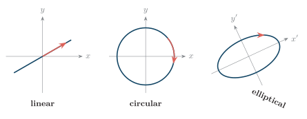
Electric-field tip trajectories for linear, circular and elliptical polarization.

How to read the figure. Each panel is a view looking along the propagation axis at one fixed observation point. The colored curve is the locus of the electric-field tip, not the path followed by the wave through space. In the linear case the vector moves back and forth on one line; in the circular and elliptical cases the arrow indicates rotation with time. The rotation direction must always be stated together with the viewing convention.

Linear Polarization

Note

Linear polarization.

A wave is linearly polarized when its electric-field tip traces a straight line. This occurs when the two orthogonal components are in phase or $180^\circ$ out of phase, or when either component is zero.

Therefore,

$$\delta=m\pi, \qquad m\in\mathbb Z,$$

where

• $\delta$ is the phase of the $y$ component relative to the $x$ component;

• $m$ is any integer: $m=0,\pm1,\pm2,\ldots$;

• $\pi$ radians equals $180^\circ$.

Thus, even $m$ means that the components are in phase, while odd $m$ means that they are $180^\circ$ out of phase.

or when either component is zero. Then the component ratio is constant:

$$\frac{E_y}{E_x} =\frac{E_{y0}}{E_{x0}}\cos\delta =\pm\frac{E_{y0}}{E_{x0}}.$$

For in-phase components, the tilt angle $\psi$ measured from the $+x$ axis is

$$\operatorname{tan}\psi=\frac{E_{y0}}{E_{x0}}.$$

Special names such as horizontal and vertical polarization depend on the chosen reference plane and antenna orientation.

Examples:

$$\mathbf E=\hat{\mathbf x}E_0\cos(\omega t-\beta z)$$

is $x$-linear, while

$$\mathbf E=E_0(\hat{\mathbf x}+\hat{\mathbf y}) \cos(\omega t-\beta z)$$

is linearly polarized at $45^\circ$ to the $x$ axis.

Circular Polarization

Note

Circular polarization.

A wave is circularly polarized when its electric-field magnitude is constant and its direction rotates uniformly, so the field tip traces a circle. It requires equal-amplitude orthogonal components in phase quadrature.

Therefore,

$$E_{x0}=E_{y0}=E_0$$

and

$$\delta=\pm\frac{\pi}{2}+2m\pi.$$

For example,

$$\mathbf E =E_0\left[ \hat{\mathbf x}\cos(\omega t-\beta z) +\hat{\mathbf y}\cos\left(\omega t-\beta z \pm\frac{\pi}{2}\right) \right].$$

Its magnitude is constant:

$$|\mathbf E| =\sqrt{E_x^2+E_y^2} =E_0.$$

Note

Circular-polarization handedness.

Under the IEEE antenna convention, observe the field in the direction of propagation: clockwise rotation is right-hand circular polarization (RHCP), and counterclockwise rotation is left-hand circular polarization (LHCP).

Because optics texts may use a different viewing convention, a careful answer states both the viewing direction and the observed rotation rather than relying on RHCP or LHCP alone.

Elliptical Polarization

Note

Elliptical polarization.

Elliptical polarization is the general state in which the electric-field tip traces an ellipse. It occurs when the orthogonal components have unequal amplitudes, a phase difference other than $0$ or $\pi$, or both.

It is specified by

• major-axis amplitude $A_{\mathrm{maj}}$;

• minor-axis amplitude $A_{\mathrm{min}}$;

• tilt angle $\psi$ of the major axis;

• rotation sense.

Note

Axial ratio.

Axial ratio $\mathrm{AR}$ is the ratio of the polarization ellipse’s major semi-axis to its minor semi-axis. It ranges from $1$ for circular polarization to infinity for linear polarization.

Its value is

$$\mathrm{AR}=\frac{A_{\mathrm{maj}}}{A_{\mathrm{min}}}, \qquad 1\le\mathrm{AR}\le\infty.$$

Therefore,

Axial ratio	Polarization
$\mathrm{AR}=1$	circular
$1<\mathrm{AR}<\infty$	elliptical
$\mathrm{AR}\to\infty$	linear

Axial ratio is sometimes stated in decibels:

$$\mathrm{AR}_{\mathrm{dB}}=20\log_{10}(\mathrm{AR}).$$

For the general component equation, the principal-axis amplitudes are

$$A_{\mathrm{maj,min}}^2 =\frac{1}{2}\left[ E_{x0}^2+E_{y0}^2 \pm \sqrt{ \left(E_{x0}^2-E_{y0}^2\right)^2 +4E_{x0}^2E_{y0}^2\cos^2\delta } \right],$$

where the plus sign gives $A_{\mathrm{maj}}^2$. The tilt angle satisfies

$$\operatorname{tan}(2\psi) =\frac{2E_{x0}E_{y0}\cos\delta} {E_{x0}^2-E_{y0}^2}.$$

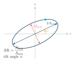
Polarization ellipse geometry.

How to read the figure. The full major and minor dimensions are $2A_{\mathrm{maj}}$ and $2A_{\mathrm{min}}$; axial ratio uses the semi-axis amplitudes, so the factor of two cancels. The dashed line shows the major-axis orientation, $\psi$ measures its tilt from the reference $x$ axis, and the arrow supplies the independent rotation-sense information. Shape, tilt and handedness are all required to describe a general ellipse.

Polarization Vector

Note

Polarization vector.

The polarization vector, or Jones vector, is a normalized complex vector whose component magnitudes and relative phases specify the polarization state.

It is

$$\hat{\mathbf p} =\frac{ \hat{\mathbf x}E_{x0} +\hat{\mathbf y}E_{y0}e^{j\delta} }{\sqrt{E_{x0}^2+E_{y0}^2}}.$$

Examples, apart from an unimportant common phase factor, are

$$\hat{\mathbf p}_x=\hat{\mathbf x}, \qquad \hat{\mathbf p}_{45^\circ} =\frac{\hat{\mathbf x}+\hat{\mathbf y}}{\sqrt2},$$

and the two opposite circular states

$$\hat{\mathbf p}_{\mathrm{c},\pm} =\frac{\hat{\mathbf x}\pm j\hat{\mathbf y}}{\sqrt2}.$$

Polarization Mismatch and Polarization Loss Factor

Maximum received power requires the receiving antenna to be matched to the incident wave’s polarization.

Note

Polarization loss factor.

The polarization loss factor (PLF) is the fraction of otherwise available received power retained after polarization mismatch. In a common complex-vector convention, it is the squared magnitude of the Hermitian inner product of the receiving and incident polarization vectors.

$$\boxed{ \mathrm{PLF} =\left| \hat{\mathbf p}_r^{\,*}\cdot\hat{\mathbf p}_i \right|^2 }$$

where $\hat{\mathbf p}_i$ describes the incident wave and $\hat{\mathbf p}_r$ describes the receiving polarization. Thus

$$0\le\mathrm{PLF}\le1.$$

Note

Polarization mismatch loss.

Polarization mismatch loss is the PLF expressed as a positive loss in decibels.

$$L_{\mathrm{pol,dB}} =-10\log_{10}(\mathrm{PLF}).$$

For two linearly polarized antennas separated by angle $\psi$,

$$\mathrm{PLF}=\cos^2\psi.$$

Polarization pair	PLF	Mismatch loss
identical linear states	$1$	$0$ dB
orthogonal linear states	$0$	ideally infinite
same-sense circular states	$1$	$0$ dB
opposite-sense circular states	$0$	ideally infinite
circular and any linear state	$1/2$	$3.01$ dB

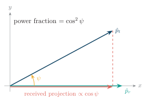
Linear polarization mismatch as a vector projection.

How to read the figure. The incident unit vector $\hat{\mathbf p}_t$ makes angle $\psi$ with the receiving axis $\hat{\mathbf p}_r$. Only its projection $\cos\psi$ produces received voltage. Since power is proportional to voltage squared, the received power fraction is $\cos^2\psi$.

Including polarization mismatch, the free-space received power is

$$P_r=P_tG_tG_r \left(\frac{\lambda}{4\pi R}\right)^2 \mathrm{PLF}.$$

Worked example: linear mismatch

A linearly polarized wave is incident at $30^\circ$ to a linearly polarized receiving antenna. Find the received power fraction and mismatch loss.

$$\mathrm{PLF}=\cos^2 30^\circ =\left(\frac{\sqrt3}{2}\right)^2 =0.75.$$

Thus the antenna receives $75\%$ of the power it would receive under perfect polarization matching, and

$$L_{\mathrm{pol,dB}} =-10\log_{10}(0.75) =1.25\ \mathrm{dB}.$$

Quick classification test

Given $E_{x0}$, $E_{y0}$ and $\delta$:

1. If one component is zero, or $\delta=0$ or $\pi$, the polarization is linear.

2. If $E_{x0}=E_{y0}$ and $\delta=\pm\pi/2$, it is circular.

3. Otherwise it is elliptical.

4. For circular or elliptical polarization, inspect the field at two increasing times to determine the rotation sense under the stated viewing convention.

Dipole Antennas

Note

Dipole antenna.

A dipole is a balanced, straight-wire antenna consisting of two conducting arms fed at or near their common centre.

Take the wire along the $z$ axis, with total length $\ell$, and measure the observation angle $\theta$ from the $+z$ axis.

Current is maximum near the feed and must fall to zero at open wire ends. The exact current distribution depends on electrical length, wire radius, feed gap and nearby objects. Radiation is therefore determined by both the total length and the current distribution.

This section uses

$$k=\frac{2\pi}{\lambda}=\omega\sqrt{\mu\varepsilon}, \qquad \eta=\sqrt{\frac{\mu}{\varepsilon}},$$

and the time convention $e^{j\omega t}$, so an outward wave contains $e^{-jkr}$.

Hertzian Current Element

Note

Hertzian dipole.

A Hertzian dipole, or infinitesimal current element, is an ideal electrically infinitesimal element carrying uniform current. It is a mathematical building block; an isolated open wire cannot carry exactly uniform current.

Its length satisfies

$$d\ell\ll\lambda$$

and it carries uniform peak phasor current $I_0$.

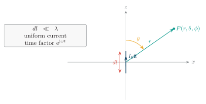
Hertzian dipole geometry.

How to read the figure. The current element $I_0d\ell\,\hat{\mathbf z}$ lies on the $z$ axis. The observation point $P(r,\theta,\phi)$ is a distance $r$ from the element, and $\theta$ is measured down from the dipole axis. Rotational symmetry about $z$ makes the fields independent of $\phi$.

Far fields

In the radiation zone, only the $1/r$ terms remain. The non-zero far-field components are

$$\boxed{ E_\theta =j\eta\frac{kI_0d\ell}{4\pi r} e^{-jkr}\sin\theta }$$

and

$$\boxed{ H_\phi=\frac{E_\theta}{\eta} =j\frac{kI_0d\ell}{4\pi r} e^{-jkr}\sin\theta. }$$

These equations show that

• $E_\theta$ and $H_\phi$ are transverse and in phase;

• both fields decrease as $1/r$;

• radiation is maximum at $\theta=90^\circ$, broadside to the wire;

• radiation is zero at $\theta=0^\circ$ and $180^\circ$, along the wire;

• there is no $\phi$ dependence.

The average far-field power density for peak phasors is

$$S_r =\frac{|E_\theta|^2}{2\eta} =\frac{\eta k^2|I_0|^2(d\ell)^2} {32\pi^2r^2}\sin^2\theta.$$

Hence the radiation intensity is

$$U(\theta) =r^2S_r =\frac{\eta k^2|I_0|^2(d\ell)^2} {32\pi^2}\sin^2\theta.$$

Total radiated power

Integrating over a sphere and using

$$\int_0^{2\pi}\int_0^\pi \sin^2\theta\sin\theta\,d\theta\,d\phi =\frac{8\pi}{3}$$

gives

$$P_{\mathrm{rad}} =\frac{\eta k^2|I_0|^2(d\ell)^2}{12\pi}.$$

In free space, $\eta_0=120\pi\ \Omega$ and $k=2\pi/\lambda$, so

$$P_{\mathrm{rad}} =40\pi^2|I_0|^2 \left(\frac{d\ell}{\lambda}\right)^2$$

for peak current. Since $P_{\mathrm{rad}}=|I_0|^2R_r/2$,

$$\boxed{ R_{r,\mathrm{Hertzian}} =80\pi^2 \left(\frac{d\ell}{\lambda}\right)^2\ \Omega. }$$

Pattern and directivity

The normalized field and power patterns are

$$F_n(\theta)=\sin\theta, \qquad P_n(\theta)=\sin^2\theta.$$

The directivity pattern is

$$D(\theta)=\frac{3}{2}\sin^2\theta,$$

so

$$D_0=1.5=1.76\ \mathrm{dBi}.$$

The power reaches one half at $\theta=45^\circ$ and $135^\circ$; therefore the elevation-plane HPBW is $90^\circ$.

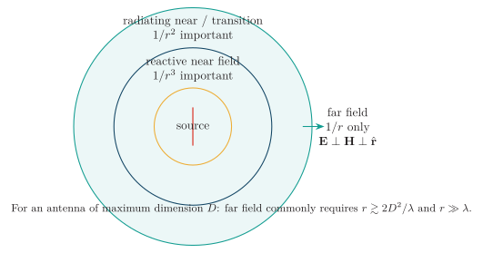
Dipole field regions.

How to read the figure. Close to the source, $1/r^3$ reactive terms can exceed the radiation term and energy is exchanged with the antenna each cycle. Through the transition region, $1/r^2$ induction terms remain important. Only in the far field does the $1/r$ term dominate, making $\mathbf E$, $\mathbf H$ and $\hat{\mathbf r}$ mutually perpendicular. The drawn boundaries are gradual field transitions, not conducting surfaces.

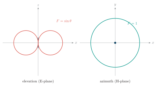
Dipole radiation patterns.

How to read the figure. The left E-plane cut contains the dipole axis and has the two-lobed field pattern $|\sin\theta|$: broadside maxima and axial nulls. The right H-plane cut is perpendicular to the dipole and is a circle because every azimuth angle $\phi$ is equivalent. Rotating the E-plane pattern about the dipole axis produces the familiar three-dimensional torus, or doughnut, pattern.

Practical Short Dipole

Note

Practical short dipole.

A practical short dipole is a centre-fed wire with total length $\ell\ll\lambda$ and an approximately triangular current distribution that falls to zero at both ends.

Its total length satisfies

$$\ell\ll\lambda,$$

but its current is approximately triangular rather than uniform:

$$I(z)\approx I_m \left(1-\frac{2|z|}{\ell}\right), \qquad -\frac{\ell}{2}\le z\le\frac{\ell}{2},$$

where $I_m$ is the peak feed current.

Note

Effective current length.

Effective current length $\ell_{\mathrm{eff}}$ is the area under the current distribution normalized to the reference current. It is the uniform-current length that gives the same current moment.

For the practical short dipole,

$$\ell_{\mathrm{eff}} =\frac{1}{I_m} \int_{-\ell/2}^{\ell/2}I(z)\,dz =\frac{\ell}{2}.$$

Therefore its far fields are obtained from the Hertzian result by replacing $I_0d\ell$ with $I_m\ell/2$:

$$E_\theta =j\eta\frac{kI_m\ell}{8\pi r} e^{-jkr}\sin\theta, \qquad H_\phi=\frac{E_\theta}{\eta}.$$

Its radiated power and radiation resistance are

$$P_{\mathrm{rad}} =10\pi^2|I_m|^2 \left(\frac{\ell}{\lambda}\right)^2$$

for peak current, and

$$\boxed{ R_{r,\mathrm{short}} =20\pi^2 \left(\frac{\ell}{\lambda}\right)^2\ \Omega. }$$

The short dipole retains the approximate $\sin\theta$ field pattern and therefore has $D_0\approx1.5$, but its very small radiation resistance makes conductor loss and impedance matching important. It is also strongly capacitive when electrically short.

Danger

Warning

Short-dipole convention. Some elementary texts use the name “short dipole” for a uniform-current element and quote $80\pi^2(\ell/\lambda)^2$. A practical centre-fed short wire has triangular current and gives $20\pi^2(\ell/\lambda)^2$. State the assumed current distribution; this removes the apparent factor-of-four contradiction.

Half-Wave Dipole

Note

Half-wave dipole.

An ideal thin half-wave dipole is a centre-fed dipole with total length $\ell=\lambda/2$ and an approximately sinusoidal current distribution.

Its length is

$$\ell=\frac{\lambda}{2}.$$

Its current is approximately sinusoidal, with maximum $I_m$ at the feed and zeros at the ends:

$$I(z)=I_m\cos(kz), \qquad -\frac{\lambda}{4}\le z\le\frac{\lambda}{4}.$$

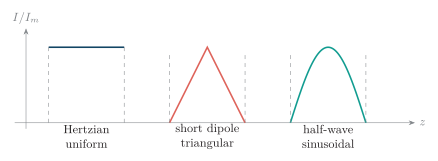
Dipole current distributions.

How to read the figure. The Hertzian model assumes constant current over its infinitesimal length. The practical short dipole has a triangular distribution and therefore half the effective current length of a uniform-current wire of the same total length. The half-wave dipole supports an approximately sinusoidal standing current. Far-field amplitude is governed by the current moment, represented here by the area under each normalized current curve.

Half-wave far fields

Integrating the contributions of all current elements gives

$$\boxed{ E_\theta =j\eta\frac{I_m e^{-jkr}}{2\pi r} \frac{\cos\!\left(\dfrac{\pi}{2}\cos\theta\right)} {\sin\theta} }$$

and

$$H_\phi=\frac{E_\theta}{\eta}.$$

Thus the normalized field pattern is

$$F_n(\theta) =\left| \frac{\cos\!\left(\dfrac{\pi}{2}\cos\theta\right)} {\sin\theta} \right|,$$

and the normalized power pattern is $P_n=F_n^2$. As for the short dipole, radiation is maximum at $\theta=90^\circ$, zero on the axis and independent of $\phi$. The half-wave elevation pattern is slightly narrower than $\sin^2\theta$.

Important half-wave values are

$$\boxed{ R_r\approx73.1\ \Omega, \qquad D_0\approx1.64=2.15\ \mathrm{dBi}, \qquad \mathrm{HPBW}\approx78^\circ. }$$

For peak feed current,

$$P_{\mathrm{rad}} =\frac{1}{2}R_r|I_m|^2 \approx36.55|I_m|^2\ \mathrm W.$$

For RMS feed current, the equivalent expression is

$$P_{\mathrm{rad}} =R_rI_{\mathrm{rms}}^2.$$

For a lossless half-wave dipole, $G_0=D_0=1.64$, and its maximum effective aperture is

$$A_{e,\max} =\frac{\lambda^2G_0}{4\pi} \approx0.1305\lambda^2.$$

Resonance and practical length

An infinitely thin dipole of exactly $\lambda/2$ has an input impedance of approximately

$$Z_A\approx73+j42.5\ \Omega.$$

It is therefore inductive, not exactly resonant. Shortening the wire cancels this reactance. A common first estimate for a practical resonant dipole is

$$\ell_{\mathrm{res}}\approx0.475\lambda.$$

Using $c\approx3\times10^8$ m/s,

$$\ell_{\mathrm{res}}\approx\frac{142.5}{f_{\mathrm{MHz}}}\ \mathrm m,$$

or approximately

$$\mathrm{each\ arm\ length}\approx \frac{71.25}{f_{\mathrm{MHz}}}\ \mathrm m.$$

The exact shortening factor depends on conductor diameter, insulation, end effects, feed arrangement and nearby objects.

Dipole Comparison

Property	Hertzian element	Practical short dipole	Half-wave dipole
Length	$d\ell\ll\lambda$	$\ell\ll\lambda$	$\ell\approx\lambda/2$
Current model	uniform	triangular	sinusoidal
Field pattern	$\sin\theta$	approximately $\sin\theta$	$\dfrac{\cos[(\pi/2)\cos\theta]}{\sin\theta}$
Radiation resistance	$80\pi^2(d\ell/\lambda)^2$	$20\pi^2(\ell/\lambda)^2$	about $73\ \Omega$
Maximum directivity	$1.5$	about $1.5$	about $1.64$
Elevation HPBW	$90^\circ$	about $90^\circ$	about $78^\circ$

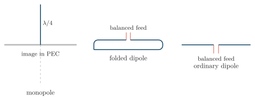
Comparison of common wire antennas.

How to read the figure. The ordinary half-wave dipole is a balanced two-arm antenna with about $73\ \Omega$ radiation resistance. A folded dipole has nearly the same pattern but, for two equal closely spaced conductors, about four times the feed resistance, roughly $4(73)=292\ \Omega$. A quarter-wave monopole above a perfect conducting ground plane uses its image as the missing arm; it radiates into the upper hemisphere and has about half the dipole feed resistance, $36.5\ \Omega$. The three drawings are conceptual and are not at a common physical scale.

Worked example: short-dipole radiation resistance

A practical short dipole has $\ell=0.05\lambda$. Its triangular-current radiation resistance is

$$R_r=20\pi^2(0.05)^2 =0.493\ \Omega.$$

If the same length were incorrectly treated as a uniform-current Hertzian element, the result would be

$$R_r=80\pi^2(0.05)^2 =1.97\ \Omega,$$

which is four times too large for the practical current distribution.

Worked example: half-wave dipole length

At $f=100$ MHz,

$$\lambda=\frac{3\times10^8}{100\times10^6} =3\ \mathrm m.$$

The ideal half-wave length is

$$\ell=\frac{\lambda}{2}=1.5\ \mathrm m,$$

while the common practical resonant estimate is

$$\ell_{\mathrm{res}}=0.475(3)=1.425\ \mathrm m.$$

Each practical arm is therefore approximately $0.7125$ m long.

Practical Antenna Types

Note

Practical antenna families.

• A wire antenna radiates from RF current distributed along one or more conducting wires; dipoles, monopoles and loops are common examples.

• A Yagi-Uda antenna is an end-fire array containing one driven element, a reflector and one or more parasitic directors.

• A log-periodic dipole array uses geometrically scaled dipoles to maintain similar impedance and radiation behavior over a wide frequency range.

• An aperture antenna radiates through an opening, such as the mouth of a horn or a slot in a conducting surface.

• A microstrip patch antenna uses a resonant conducting patch above a ground plane, separated by a dielectric substrate.

• A helical antenna is a conducting helix that can operate in normal mode or produce a directional, approximately circularly polarized beam in axial mode.

• A reflector antenna uses a conducting reflecting surface to redirect radiation from a feed into a more directive beam.

These families differ mainly by bandwidth, directivity, size, polarization and feeding method.

The family map groups antennas by the physical structure and radiation mechanism that dominate their behavior.

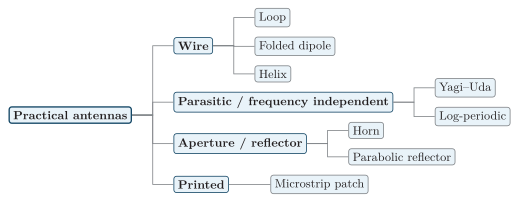
Practical antenna families organized by wire, parasitic, frequency-independent, aperture, reflector, and printed structures.

Wire geometry controls both the radiation pattern and the feed-point impedance.

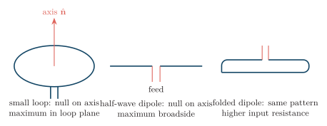
Small-loop, half-wave-dipole, and folded-dipole wire antennas with their principal radiation directions.

A Yagi-Uda obtains directional gain through coupling between one driven element and several parasitic elements.

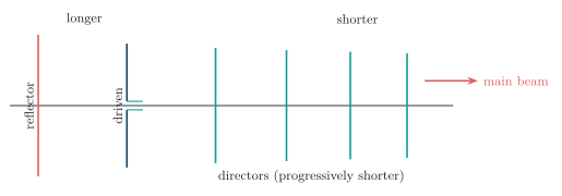
Yagi-Uda antenna with a reflector, driven element, progressively shorter directors, and a forward main beam.

The driven element is normally a half-wave or folded dipole. A slightly longer reflector is placed behind it, while one or more shorter directors are placed toward the desired beam. Mutual coupling induces currents in these parasitic elements; their lengths and spacings make the reradiated fields add toward the directors and partly cancel behind the reflector. More directors usually increase gain and narrow the beam, with diminishing improvement per element. A conventional Yagi is therefore directional and efficient but narrower-band than a log-periodic array.

A log-periodic array repeats a scaled geometry so that different element groups become active at different frequencies.

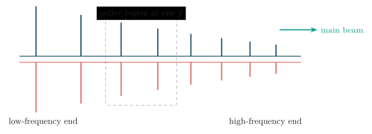
Log-periodic dipole array whose self-similar element progression supports wideband operation.

Horn and reflector antennas use aperture geometry and focusing to produce high directivity.

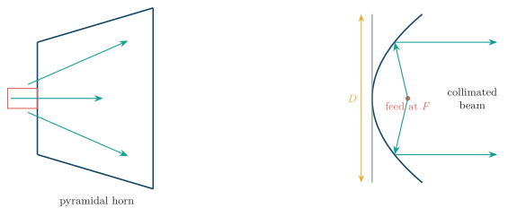
Pyramidal-horn and focus-fed parabolic-reflector antennas forming collimated beams.

A microstrip patch radiates mainly from fringing fields at the open edges of the resonant conductor.

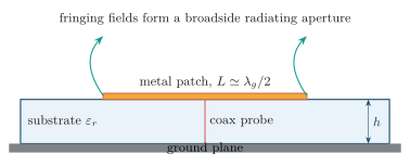
Probe-fed microstrip patch above a dielectric substrate and ground plane, with radiation from edge fringing fields.

In axial mode, a helix supports a travelling wave and produces an approximately circularly polarized end-fire beam.

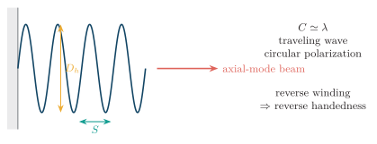
Axial-mode helical antenna showing circumference, turn spacing, travelling wave, and end-fire radiation.

Antenna selection is therefore a trade-off among bandwidth, gain, profile, polarization, and operating band.

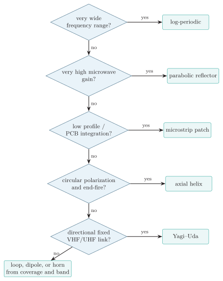
Decision flow for selecting an antenna family from bandwidth, gain, profile, polarization, and link requirements.

VHF Antenna Selection

The very-high-frequency band extends from $30$ to $300\ \mathrm{MHz}$, corresponding to wavelengths from about $10$ to $1\ \mathrm m$. Common choices include half-wave and folded dipoles, quarter-wave monopoles, Yagi-Uda arrays, log-periodic dipole arrays, collinear vertical arrays and crossed dipoles. The choice depends on coverage direction, bandwidth, polarization, available space, wind loading and feeder impedance.

Since $G=\eta_rD$, VHF gain can be improved in two distinct ways:

• Increase directivity with a longer Yagi, a larger array aperture, stacked antennas, a collinear array, a reflector or an appropriate feed-phase progression.

• Increase radiation and realized efficiency with low-resistance conductors, low-loss feed line, sound joints, a suitable balun, correct impedance matching and clearance from detuning objects.

Higher gain redistributes the available radiation into a narrower angular region; it does not create transmitter power. Greater mounting height may improve the radio horizon without changing the antenna’s intrinsic gain.

A parabolic reflector is electromagnetically possible at VHF, but useful gain requires a very large aperture because

$$G\approx\eta_a\left(\frac{\pi D}{\lambda}\right)^2.$$

At $100\ \mathrm{MHz}$, $\lambda=3\ \mathrm m$. For $20\ \mathrm{dBi}$ gain, $G=100$, and aperture efficiency $\eta_a=0.6$,

$$D=\frac{\lambda}{\pi}\sqrt{\frac{G}{\eta_a}} \approx12.3\ \mathrm m.$$

Such a dish has substantial cost, wind load and steering requirements. Yagi, log-periodic or stacked arrays are therefore usually more practical for VHF, while very large reflectors remain useful in specialized installations such as radio astronomy.

Antenna Arrays

Note

Antenna array.

An antenna array is a group of radiating elements whose relative positions, excitation amplitudes and phases are selected to produce a desired combined radiation pattern.

For a uniform linear array, the path difference to a distant observation point determines the relative phase of each element contribution.

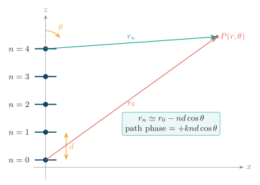
Uniform linear array geometry showing element spacing, observation angle, path difference, and phase progression.

Element spacing and feed phase determine whether a two-element array radiates broadside or end-fire.

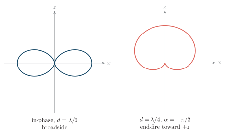
Broadside and end-fire patterns produced by different spacing and phase conditions in a two-element array.

A linear feed-phase gradient rotates the equal-phase front and steers the main beam without moving the array.

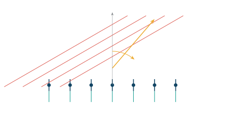
Electronic beam steering by a progressive phase shift across the elements of a linear array.

Amplitude taper reduces sidelobes at the cost of a wider main beam and lower peak directivity.

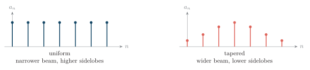
Uniform and tapered element excitation, illustrating the trade-off between beamwidth and sidelobe level.