Electromagnetic Waves and Materials

Wave Equation

Note

Electromagnetic wave equation.

The electromagnetic wave equation is the second-order differential equation obtained from Maxwell’s curl equations that describes the spatial and temporal propagation of electric and magnetic fields through a medium.

In a source-free, linear, homogeneous medium,

$$\nabla\times\mathbf{E}=-\mu\frac{\partial\mathbf{H}}{\partial t}, \qquad \nabla\times\mathbf{H}=\sigma\mathbf{E}+\varepsilon\frac{\partial\mathbf{E}}{\partial t}.$$

For a source-free homogeneous medium, Gauss’s laws and the constant material parameters imply

$$\nabla\cdot\mathbf E=0, \qquad \nabla\cdot\mathbf H=0.$$

These conditions remove the gradient-divergence terms when the double-curl identity is applied.

Note

Derivation: Electric-field wave equation

Take the curl of Faraday’s law:

$$\nabla\times(\nabla\times\mathbf{E}) =-\mu\frac{\partial}{\partial t}(\nabla\times\mathbf{H}).$$

Substitute the Ampere-Maxwell law into the right-hand side:

$$\begin{aligned} \nabla\times(\nabla\times\mathbf{E}) & =-\mu\frac{\partial}{\partial t} \left(\sigma\mathbf{E}+\varepsilon\frac{\partial\mathbf{E}}{\partial t}\right) \\ & =-\mu\sigma\frac{\partial\mathbf{E}}{\partial t} -\mu\varepsilon\frac{\partial^2\mathbf{E}}{\partial t^2}. \end{aligned}$$

Use the vector identity

$$\nabla\times(\nabla\times\mathbf{E}) =\nabla(\nabla\cdot\mathbf{E})-\nabla^2\mathbf{E}.$$

In a source-free homogeneous medium, Gauss’s law and $\mathbf{D}=\varepsilon\mathbf{E}$, with constant $\varepsilon$, give

$$0=\nabla\cdot\mathbf{D} =\nabla\cdot(\varepsilon\mathbf{E}) =\varepsilon\nabla\cdot\mathbf{E} \quad\Longrightarrow\quad \nabla\cdot\mathbf{E}=0.$$

Therefore,

$$-\nabla^2\mathbf{E} =-\mu\sigma\frac{\partial\mathbf{E}}{\partial t} -\mu\varepsilon\frac{\partial^2\mathbf{E}}{\partial t^2}.$$

The resulting electric-field wave equation is

$$\boxed{ \nabla^2\mathbf{E}=\mu\sigma\frac{\partial\mathbf{E}}{\partial t} +\mu\varepsilon\frac{\partial^2\mathbf{E}}{\partial t^2}. }$$

For a lossless medium, $\sigma=0$:

$$\nabla^2\mathbf{E}-\mu\varepsilon\frac{\partial^2\mathbf{E}}{\partial t^2}=0.$$

Note

Derivation: Magnetic-field wave equation

To obtain the magnetic-field wave equation, combine the same two Maxwell curl equations in the opposite order. Take the curl of the Ampere-Maxwell law:

$$\begin{aligned} \nabla\times(\nabla\times\mathbf{H}) & =\sigma(\nabla\times\mathbf{E}) +\varepsilon\frac{\partial}{\partial t}(\nabla\times\mathbf{E}). \end{aligned}$$

Substitute Faraday’s law, $\nabla\times\mathbf{E}=-\mu\partial\mathbf{H}/\partial t$:

$$\nabla\times(\nabla\times\mathbf{H}) =-\mu\sigma\frac{\partial\mathbf{H}}{\partial t} -\mu\varepsilon\frac{\partial^2\mathbf{H}}{\partial t^2}.$$

Use the vector identity

$$\nabla\times(\nabla\times\mathbf{H}) =\nabla(\nabla\cdot\mathbf{H})-\nabla^2\mathbf{H}.$$

For constant $\mu$, Gauss’s law for magnetism gives

$$0=\nabla\cdot\mathbf{B} =\nabla\cdot(\mu\mathbf{H}) =\mu\nabla\cdot\mathbf{H} \quad\Longrightarrow\quad \nabla\cdot\mathbf{H}=0.$$

Therefore,

$$\boxed{ \nabla^2\mathbf{H} =\mu\sigma\frac{\partial\mathbf{H}}{\partial t} +\mu\varepsilon\frac{\partial^2\mathbf{H}}{\partial t^2} }.$$

For a lossless medium, $\sigma=0$:

$$\boxed{ \nabla^2\mathbf{H} -\mu\varepsilon\frac{\partial^2\mathbf{H}}{\partial t^2}=0 }.$$

Uniform Plane Waves

Note

Uniform plane wave.

A uniform plane wave has electric and magnetic fields that are constant over every plane normal to the propagation direction; $\mathbf E$, $\mathbf H$ and the propagation direction are mutually perpendicular.

For a wave travelling in the $+z$ direction,

$$\mathbf{E}=E_0\cos(\omega t-\beta z)\mathbf{a}_x, \qquad \mathbf{H}=H_0\cos(\omega t-\beta z)\mathbf{a}_y.$$

Symbols used:

Symbol	Meaning	SI unit
$\mathbf{E}(z,t)$	Instantaneous electric-field vector	$\mathrm{V/m}$
$\mathbf{H}(z,t)$	Instantaneous magnetic-field-intensity vector	$\mathrm{A/m}$
$E_0$	Peak electric-field amplitude	$\mathrm{V/m}$
$H_0$	Peak magnetic-field amplitude	$\mathrm{A/m}$
$\omega=2\pi f$	Angular frequency, where $f$ is frequency	$\mathrm{rad/s}$
$t$	Time	$\mathrm{s}$
$\beta=2\pi/\lambda$	Phase constant, where $\lambda$ is wavelength	$\mathrm{rad/m}$
$z$	Position measured along the propagation axis	$\mathrm{m}$
$\mathbf{a}_x$	Unit vector in the $+x$ direction; direction of $\mathbf E$	dimensionless
$\mathbf{a}_y$	Unit vector in the $+y$ direction; direction of $\mathbf H$	dimensionless
$\omega t-\beta z$	Wave phase; the minus sign indicates propagation in $+z$	$\mathrm{rad}$

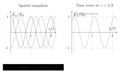
Time-domain snapshots of a propagating sinusoidal wave.

How to read the figure. The left panel holds time fixed and shows the spatial waveform at successive instants; the right panel holds position fixed and shows the field oscillating in time. The spatial period is $\lambda=2\pi/\beta$, the time period is $T=2\pi/\omega$, and the phase $\omega t-\beta z$ advances in the $+z$ direction.

The propagation direction is

$$\mathbf{E}\times\mathbf{H}.$$

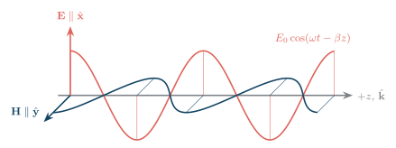
Uniform plane wave with mutually perpendicular electric field, magnetic field and propagation direction.

How to read the figure. The wave travels along $+z$, while $\mathbf E$ points along $x$ and $\mathbf H$ points along $y$. Thus $\mathbf E\perp\mathbf H$, both fields are transverse to the propagation axis, and $\mathbf E\times\mathbf H$ points in the direction of travel.

Note

Wave velocity, phase constant and intrinsic impedance.

Wave velocity $v$ is the speed of phase propagation, phase constant $\beta$ is phase change per unit distance, and intrinsic impedance $\eta$ is the electric-to-magnetic field ratio of a travelling wave in the medium.

In a lossless medium,

$$v=\frac{1}{\sqrt{\mu\varepsilon}}, \qquad \beta=\omega\sqrt{\mu\varepsilon}, \qquad \eta=\frac{E}{H}=\sqrt{\frac{\mu}{\varepsilon}}.$$

In free space,

$$c=\frac{1}{\sqrt{\mu_0\varepsilon_0}}, \qquad \eta_0=\sqrt{\frac{\mu_0}{\varepsilon_0}}\approx377\ \Omega.$$

Note

Intrinsic impedance of a dielectric

For a lossless dielectric with $\mu_r=1$ and $\varepsilon_r=4$,

$$\eta=\eta_0\sqrt{\frac{\mu_r}{\varepsilon_r}} =377\sqrt{\frac{1}{4}} =188.5\ \Omega.$$

The magnetic-field amplitude is therefore $H=E/188.5$ for a travelling plane wave in this medium.

Power Flow and Energy

Note

Poynting vector.

The Poynting vector $\mathbf S$ is electromagnetic power flow per unit area; its direction gives the local direction of energy transport.

Its instantaneous value is

$$\mathbf{S}=\mathbf{E}\times\mathbf{H}.$$

For phasors,

$$\mathbf{S}_{\text{av}}=\frac{1}{2}\operatorname{Re}\left(\mathbf{E}\times\mathbf{H}^*\right).$$

The average power crossing a surface $A$ is the normal flux of $\mathbf S_{\text{av}}$:

$$P_{\text{av}}=\int_A\mathbf S_{\text{av}}\cdot d\mathbf S.$$

For a uniform wave incident at angle $\theta$ to the surface normal,

$$P_{\text{av}}=S_{\text{av}}A\cos\theta.$$

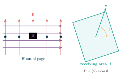
Power flow for oblique fields.

How to read the figure. Only the component of $\mathbf S_{\text{av}}$ parallel to the area normal crosses the receiving surface. The collected power is maximum at normal incidence and decreases by the projection factor $\cos\theta$.

A coaxial line gives a practical example of the cross product $\mathbf S=\mathbf E\times\mathbf H$.

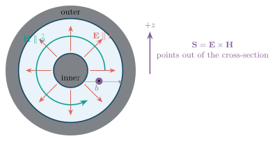
Power flow in a coaxial line.

How to read the figure. Between the conductors, $\mathbf E$ is radial and $\mathbf H$ is azimuthal, so their cross product points along the cable. Electromagnetic energy is transported through the dielectric between the conductors.

Note

Electric and magnetic energy densities.

Electric energy density $w_e$ and magnetic energy density $w_m$ are the electromagnetic energies stored per unit volume in the electric and magnetic fields.

For linear media,

$$w_e=\frac{1}{2}\varepsilon E^2, \qquad w_m=\frac{1}{2}\mu H^2.$$

Note

Poynting theorem.

The net electromagnetic power entering a volume equals the rate of increase of stored field energy plus the power converted to heat or work inside the volume.

With $d\mathbf S$ directed outward,

$$-\oint_{\partial V}\mathbf S\cdot d\mathbf S =\frac{d}{dt}\int_V(w_e+w_m)\,dV +\int_V\mathbf J\cdot\mathbf E\,dV.$$

Equivalently,

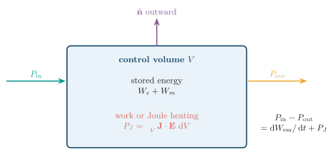
$$P_{\text{in}}-P_{\text{out}} =\frac{dW_{\text{em}}}{dt}+P_J.$$

Poynting theorem control volume.

How to read the figure. Power entering the control volume either increases the stored electric and magnetic energy or is transferred to matter through $P_J=\int_V\mathbf J\cdot\mathbf E\,dV$; any remaining power leaves the volume.

Material Parameters

Permittivity vs Permeability

Aspect	Permittivity	Permeability
Quantity and field relation	$\varepsilon$; $\mathbf D=\varepsilon\mathbf E$	$\mu$; $\mathbf B=\mu\mathbf H$
Physical meaning	Relates electric flux density to electric field and indicates how strongly the medium polarizes	Relates magnetic flux density to magnetic field and indicates how strongly the medium supports magnetic flux
SI unit	farad per metre, $\mathrm{F/m}$	henry per metre, $\mathrm{H/m}$
Relative value and meaning	$\varepsilon_r=\varepsilon/\varepsilon_0$: electric response relative to vacuum; for the same $\mathbf E$, the material has $\varepsilon_r$ times the vacuum electric flux density	$\mu_r=\mu/\mu_0$: magnetic response relative to vacuum; for the same $\mathbf H$, the material has $\mu_r$ times the vacuum magnetic flux density
Free-space reference	$\varepsilon_0\approx8.854\times10^{-12}\ \mathrm{F/m}$ and $\varepsilon_r=1$	$\mu_0\approx1.257\times10^{-6}\ \mathrm{H/m}$ and $\mu_r=1$

Conductivity.

Note

Note

Conductivity $\sigma$ describes how readily a medium supports conduction current: $\mathbf J=\sigma\mathbf E$. Its SI unit is siemens per metre ($\mathrm{S/m}$), and ideal free space has $\sigma=0$.

Loss tangent

Note

Note

Loss tangent $\tan\delta$ is the ratio of conduction current density to displacement current density in a lossy dielectric and indicates the relative importance of dielectric loss. For a medium represented by $\sigma$, $\varepsilon$ and angular frequency $\omega$, $\tan\delta=\frac{\sigma}{\omega\varepsilon}$

Propagation Constant and Intrinsic Impedance

Note

Propagation constant.

The complex propagation constant $\gamma=\alpha+j\beta$ governs a wave’s variation with distance: $\alpha$ is attenuation in nepers per metre and $\beta$ is phase change in radians per metre.

The propagation constant is

$$\boxed{ \gamma=\alpha+j\beta =\sqrt{j\omega\mu(\sigma+j\omega\varepsilon)} }.$$

With the $e^{j\omega t}$ convention, the reusable phasor differentiation rules are

$$\frac{\partial}{\partial t}\longrightarrow j\omega, \qquad \frac{\partial^2}{\partial t^2}\longrightarrow-\omega^2.$$

Note

Derivation: Propagation constant

Start with the time-domain electric-field wave equation derived earlier:

$$\nabla^2\mathbf E =\mu\sigma\frac{\partial\mathbf E}{\partial t} +\mu\varepsilon\frac{\partial^2\mathbf E}{\partial t^2}.$$

Write $\mathbf E(\mathbf r,t)=\operatorname{Re}\{\widetilde{\mathbf E}(\mathbf r)e^{j\omega t}\}$ and apply the phasor differentiation rules above. The time-domain wave equation becomes

$$\begin{aligned} \nabla^2\widetilde{\mathbf E} & =j\omega\mu\sigma\widetilde{\mathbf E} -\omega^2\mu\varepsilon\widetilde{\mathbf E} \\ & =j\omega\mu(\sigma+j\omega\varepsilon)\widetilde{\mathbf E}. \end{aligned}$$

Define

$$\gamma^2=j\omega\mu(\sigma+j\omega\varepsilon).$$

The phasor wave equation is then

$$\nabla^2\widetilde{\mathbf E}-\gamma^2\widetilde{\mathbf E}=0.$$

For a uniform plane wave varying only with $z$,

$$\frac{d^2\widetilde{\mathbf E}}{dz^2}-\gamma^2\widetilde{\mathbf E}=0,$$

To connect $\alpha+j\beta$ directly to the square root, expand both sides of $\gamma^2=j\omega\mu(\sigma+j\omega\varepsilon)$:

$$(\alpha+j\beta)^2 =(\alpha^2-\beta^2)+j2\alpha\beta =-\omega^2\mu\varepsilon+j\omega\mu\sigma.$$

Equating real and imaginary parts gives

$$\alpha^2-\beta^2=-\omega^2\mu\varepsilon, \qquad 2\alpha\beta=\omega\mu\sigma.$$

Thus $\alpha$ controls attenuation and $\beta$ controls phase progression; together they form the complex square root above.

For a passive medium, choose the square-root branch with $\alpha\ge0$ so that field amplitude does not grow with propagation distance. The general one-dimensional solution is

$$\widetilde{\mathbf E}(z) =\mathbf E_0^+e^{-\gamma z}+\mathbf E_0^-e^{\gamma z},$$

where the first term travels in $+z$ and the second travels in $-z$.

For propagation in the $+z$ direction,

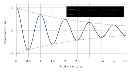
$$\widetilde E(z)=E_0e^{-\gamma z}=E_0e^{-\alpha z}e^{-j\beta z}, \qquad E(z,t)=E_0e^{-\alpha z}\cos(\omega t-\beta z).$$

Attenuating wave in a lossy medium.

How to read the figure. The sinusoid continues to advance in phase according to $\beta$, while its upper and lower envelopes shrink as $e^{-\alpha z}$. Thus $\alpha$ controls amplitude loss and $\beta$ controls phase change.

Note

Complex intrinsic impedance.

Complex intrinsic impedance $\eta_c$ is the phasor ratio of electric to magnetic field for a travelling wave in a lossy medium; its magnitude and phase describe the relative field amplitudes and phase shift.

It is

$$\eta_c=\sqrt{\frac{j\omega\mu}{\sigma+j\omega\varepsilon}}.$$

Types of Media

Note

Electromagnetic medium classes.

A perfect dielectric has $\sigma=0$, a lossless medium has no attenuation, a lossy dielectric has finite conduction loss, and a good conductor satisfies $\sigma\gg\omega\varepsilon$ so its fields decay rapidly with depth.

Medium	Condition	Main result
Perfect dielectric	$\sigma=0$	$\alpha=0$, $\eta$ real
Lossless medium	no conduction loss	phase changes, amplitude constant
Lossy dielectric	finite $\sigma$	attenuation and phase shift both occur
Good conductor	$\sigma\gg\omega\varepsilon$	field decays rapidly with depth

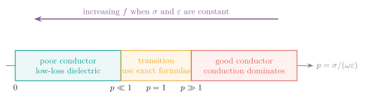
Medium regimes classified by conductivity and frequency.

How to read the figure. Move from left to right as $p=\sigma/(\omega\varepsilon)=\tan\delta$ increases: displacement current dominates for $p\ll1$, neither term may be neglected near $p=1$, and conduction current dominates for $p\gg1$. If $\sigma$ and $\varepsilon$ remain constant, increasing frequency moves the material toward the left.

Note

Good conductor.

At a specified frequency, a good conductor is a medium in which conduction current greatly exceeds displacement current, $\sigma\gg\omega\varepsilon$.

For a good conductor,

$$\alpha\approx\beta\approx\sqrt{\pi f\mu\sigma}, \qquad \eta_c\approx(1+j)\sqrt{\frac{\omega\mu}{2\sigma}}.$$

Wave Interfaces

Note

Wave interface.

A wave interface is a boundary between media; when their wave impedances differ, an incident wave generally divides into reflected and transmitted waves while satisfying electromagnetic boundary conditions.

Normal Incidence

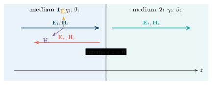
For a wave incident normally from medium 1 onto medium 2, the electric-field reflection and transmission coefficients are

$$\Gamma=\frac{E_{r0}}{E_{i0}} =\frac{\eta_2-\eta_1}{\eta_2+\eta_1}, \qquad au=\frac{E_{t0}}{E_{i0}} =\frac{2\eta_2}{\eta_1+\eta_2}=1+\Gamma.$$

Normal incidence on an impedance discontinuity.

How to read the figure. The incident wave approaches the boundary in medium 1, the reflected wave returns through medium 1, and the transmitted wave continues through medium 2. The impedance change determines their amplitude ratios through $\Gamma$ and $\tau$.

Perfect Electric Conductor

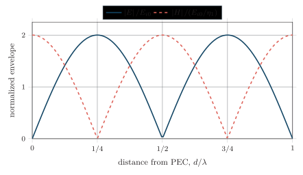
For a perfect electric conductor, $\eta_2\to0$ and hence $\Gamma=-1$. The tangential electric field vanishes at the surface, and the incident and reflected waves form standing-wave envelopes:

$$\frac{|E(d)|}{E_{i0}}=2|\sin(\beta_1d)|, \qquad \frac{|H(d)|}{E_{i0}/\eta_1}=2|\cos(\beta_1d)|.$$

Standing-wave envelopes at a perfect electric conductor.

How to read the figure. At the conductor surface, $d=0$, the electric field has a node and the magnetic field has an antinode. Their neighboring extrema are separated by $\lambda/4$.

Oblique Incidence

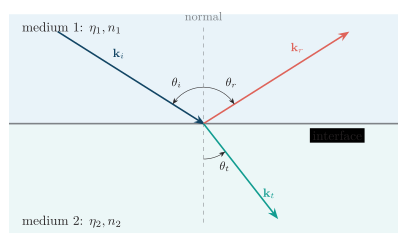
At oblique incidence, the law of reflection and Snell’s law are

$$\displaystyle\theta_r=\theta_i, \qquad n_1\sin\theta_i=n_2\sin\theta_t.$$

Oblique reflection and refraction at a plane boundary.

How to read the figure. The incident, reflected, and transmitted wave vectors lie in the plane of incidence. Every angle is measured from the interface normal, not from the interface itself.

Skin Effect

Note

Skin effect and skin depth.

Skin effect is the concentration of alternating current and electromagnetic fields near a conductor surface. Skin depth $\delta_s$ is the distance into the conductor at which field or current-density amplitude falls to $1/e$ of its surface value.

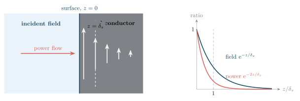
Inside a conductor, field and current density decrease approximately as

$$J(z)=J_0e^{-z/\delta_s}.$$

For a good conductor, $\sigma\gg\omega\varepsilon$, so its propagation constant reduces to

$$\gamma\approx\sqrt{j\omega\mu\sigma} =(1+j)\sqrt{\frac{\omega\mu\sigma}{2}}.$$

Hence

$$\alpha\approx\beta\approx\sqrt{\frac{\omega\mu\sigma}{2}}.$$

Defining skin depth by $e^{-\alpha\delta_s}=e^{-1}$ gives

Skin depth is

$$\delta_s=\frac{1}{\alpha}=\sqrt{\frac{2}{\omega\mu\sigma}} =\frac{1}{\sqrt{\pi f\mu\sigma}}.$$

Higher frequency, permeability or conductivity gives smaller skin depth.

Note

Copper skin depth at $5\ \mathrm{MHz}$

For copper, take $\sigma=5.8\times10^7\ \mathrm{S/m}$ and $\mu_r\approx1$. Then

$$\begin{aligned} \delta_s & =\frac{1}{\sqrt{\pi f\mu_0\sigma}} \\ & =\frac{1}{\sqrt{\pi(5\times10^6) (4\pi\times10^{-7})(5.8\times10^7)}} \\ & \approx2.96\times10^{-5}\ \mathrm m =29.6\ \mu\mathrm m. \end{aligned}$$

For the same material, $\delta_s\propto1/\sqrt f$; doubling frequency reduces the skin depth by $1/\sqrt2$.

Skin depth in a conducting medium.

How to read the figure. At $z=\delta_s$, field and current-density amplitudes have fallen to $e^{-1}$ of their surface values. Power is proportional to field amplitude squared, so it falls as $e^{-2z/\delta_s}$.

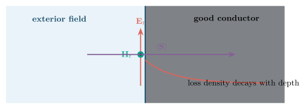
For sinusoidal fields in a conductor, the average Joule-loss density is

$$p_{J,\text{av}}(z) =\frac{1}{2}\sigma|\widetilde E(z)|^2 \propto e^{-2z/\delta_s}.$$

Power penetration and loss under skin effect.

How to read the figure. Average Poynting flux crosses the conductor surface and is converted to Joule heat. Because the fields decay rapidly with depth, most of this loss is concentrated within a few skin depths of the surface.

Because the effective current-carrying area shrinks with frequency, AC resistance, feeder attenuation, conductor heating and waveguide-wall loss all increase. RF conductors therefore use smooth, highly conductive surfaces, low-resistance joints and adequate circumference. Silver plating can reduce surface resistance, hollow conductors avoid unused bulk at microwave frequencies, and Litz wire can reduce skin and proximity effects at lower RF frequencies.